Backyard Worlds: Cool Neighbors – Explore the Mysteries of Extreme Brown Dwarfs

The Cool Neighbors logo, designed by Matteo Gulla. Feel free to share it and help spread the word!

Happy first week of Summer! We’re eager to begin the season by announcing an exciting new project: Backyard Worlds: Cool Neighbors. My name is Grady Robbins, a core member of the Cool Neighbors team, and I am thrilled to introduce our project. Stay with us to learn more about our team, the project, and how you can participate in exciting discoveries of extreme brown dwarfs.

What is Backyard Worlds: Cool Neighbors?

Backyard Worlds: Cool Neighbors focuses on finding brown dwarfs in the Sun’s cosmic neighborhood through a crowdsourced approach. Brown dwarfs are solitary substellar objects with masses between those of the most massive planets (like Jupiter) and the least massive stars (known as red dwarfs). Although brown dwarfs lack sufficient mass to sustain hydrogen fusion, as a star would, brown dwarfs still glow faintly, slowly giving off the heat from their initial formation over billions of years. Consequently, brown dwarfs emit only a small amount of light, primarily infrared light.

You might wonder why it’s so crucial to discover brown dwarfs. Here’s the exciting part: their atmospheres closely resemble those of giant exoplanets but without a brighter host star’s interference — brown dwarf atmospheres can have clouds and water! Studying these atmospheres can deepen our understanding of the development of molecules such as water and methane which are vital for the emergence of life. Some brown dwarfs may even be rogue planets ejected from their star systems! Unraveling the mysteries of these cosmic nomads provides insight into the formation of star and planet systems.

Dramatic Dwarf Discoveries

The Backyard Worlds project has already achieved remarkable breakthroughs in the study of brown dwarfs, leading to the identification of new brown dwarf classes! Recently, the project made sensational discoveries, including the identification of two extraordinary T-type subdwarfs and an intriguing new Y-dwarf. Notably, extreme T-type subdwarfs are incredibly rare due to their exceptionally low metallicity, which explains why the discoveries of the first extreme T-type brown dwarfs (WISEA 0414−5854 and WISEA 1810−1010) were not made until 2020 by the Backyard Worlds project!

One of the most remarkable findings was the first Y-dwarf (WISE 1534–1043), fittingly named “The Accident”. This discovery, stumbled upon by citizen scientist Dan Caselden through a program he built, drew significant attention. Y-dwarfs represent the coldest of brown dwarfs, making them particularly challenging to detect. The Accident, likely metal-poor and old, has even been selected for observation by the James Webb Space Telescope (JWST). It’s fascinating to think that a brown dwarf you discover could potentially be observed by JWST!

Cool Neighbors hopes to find more bizarre brown dwarf targets, like The Accident, for JWST to observe. Credit: ESA

The Backyard Worlds: Cool Neighbors project is led by Dr. Aaron Meisner, well-known for his extensive search in Backyard Worlds: Planet 9 by utilizing data from the Wide-field Infrared Survey Explorer (WISE). Developed by NOIRLab interns Austin Humphreys, Noah Schapera, and myself, the project underwent a successful beta test prior to launch, heightening expectations for future results! The project is funded and supported by NASA’s Citizen Science Seed Funding Program (CSSFP) and NSF’s NOIRLab, giving a solid foundation. This support has even facilitated the creation of multiple internships and enabled new research in astronomy!

The Accident is a prime example of the types of brown dwarfs that Backyard Worlds: Cool Neighbors aims to uncover. While The Accident was stumbled upon, the advanced search capabilities offered by Cool Neighbors are expected to reveal many more like it! The project benefits from nine years of WISE observations, enabling the discovery of even fainter brown dwarfs than ever before! Cool Neighbors uses citizen science to sift through telescope data and identify brown dwarfs hidden among stars, galaxies, and detector noise. Although the machine-learning algorithm significantly reduces the search effort to find potential brown dwarfs, it can still be deceived by artifacts and noise that mimic movement (which is precisely why your contribution is crucial)! With your help, we can potentially uncover hundreds to thousands of previously unknown substellar objects!

Search Kickoff: Where to Begin?

To start searching for brown dwarfs, visit our website at http://coolneighbors.org and click on the “CLASSIFY” tab. This opens a classification workflow, enabling you to carefully analyze images and determine if the objects you see might be brown dwarfs. The interactive interface allows you to zoom, pan, and animate to detect movement. We provide a comprehensive tutorial and a field guide to enhance your understanding and assist you in making remarkable celestial discoveries.

When you identify a potential brown dwarf, we encourage you to use the powerful astronomical databases SIMBAD and VizieR to check if the object has been published before. These databases, commonly used by professional astronomers, help determine whether your find is a new discovery or a known object. If you find a mover not listed in SIMBAD, we’d be thrilled to hear about it through our submission form or on our Zooniverse Talk page.

Backyard Worlds: Cool Neighbors offers an opportunity to contribute to cutting-edge scientific research and be part of the journey to understand the mysteries of our cosmic neighborhood. Explore our project and leave your mark on the frontiers of scientific discovery! Together, we can unveil the secrets hidden within our cosmic neighborhood and expand our understanding of the universe we call home.

Hope to see you out there,

The Cool Neighbors team

Una guía para clasificar en “BackyardWorlds: Planet 9” desde el punto devista de un científico ciudadano.

(Thanks to Paula Pancorbo Pabo for this translation! Here you can find the original article, by Michaela Allen, featuring a video by Guillaume Colin!)

¡Hola recién llegados a Backyard Worlds: Planet 9! O quizás eres un cuidadano científico que regresa a este proyecto…En cualquier caso, ¡bienvenido! Mi objetivo en esta publicación es ofreceros una guiá básica de principiantes para clasificar objetos en BW (Backyard Worlds: Planet 9) No soy una experta, pero me gustaría compartir lo que he estado aprendiendo para que quizás vosotros también podáis aprender algo.

Pero antes de empezar os voy a contar un poco sobre mí…Me llamo Michaela Allen, y estoy estudiando física y astronomía en la universidad. He estado ayudando a clasificar objetos en BW desde que empezó el proyecto y he aprendido mucho desde entonces. Al empezar en este proyecto, no tenía ni
idea de qué implicaba, sólo estaba emocionada por la posibilidad de encontrar algo que jamás se hubiese descubierto antes.

Lo primero que me gustaría compartir con todo el mundo es un video de youtube hecho por un un compañero ciudadano científico, Guillaume Colin, con todo sobre su método de analizar flipbooks en BW. Es un gran video donde habla de las bases de BW, SIMBAD e IRSA. También está detrás de los pasos para rellenar el formulario “creo que he encontrado algo” ya que puede resultar
algo complicado encontrar toda la información para el formulario. De verdad, echadle un vistazo. ¡Y gracias a Guillaume por hacer este video!

Ahora, para el resto del artículo, vamos a repasar algunos de mis temas favoritos de BW. ¡Empecemos!

Cuando entras en BW ves un tutorial que muestra diferentes ejemplos de dipolos, movers/movedizos, artefactos, etc. También tienes una guía practica a la derecha de la pantalla que muestra estos ejemplos. Tanto el tutorial como la guía con excelentes referencias para mirar una y otra vez. ¡No olvides consultarlos! Si bien estas herramientas son muy útiles para empezar, hacer tu primera clasificación puede resultar abrumador. Me gustaría daros algunos ejemplos más de tipos de objetos que podríais encontrar mientras clasificáis.

En lo que concierne a movedizos rápidos, aun no he encontrado ninguno. El ejemplo de la guía, la enana de tipo Y WISE 0855-0714 sigue siendo mi referente. Y recordad, un verdadero movedizo rápido aparecerá en los cuatro fotogramas del sujeto.

Este sujeto contiene un tipo de artefacto llamado fantasma y sólo aparece en dos fotogramas. Estos fantasmas no se mueven y no es necesario reportarlos en el formulario. Otro impostor a tener en cuenta es el ruido adicional que aparece en el área de la Anomalía del Atlántico Sur. Se encuentra a -25 grados de declinación (con un margen de unos pocos minutos de arco) Esta anomalía es de la que más habla Marc en su artículo sobre movedizos rápidos, donde tiende a causar mucho más ruido en los sujetos, y este ruido puede parecerse mucho a los movedizos rápidos.

También hay un par de puntos naranjas visibles a lo largo de los fotogramas, los cuales se pueden malinterpretar como movedizos rápidos, pero es sólo ruido. El área de declinación y el movimiento, a veces esporádico, de estos puntos nos revelan que no son movedizos. En términos de dipolos o movedizos lentos he observado muchos. Algunos definitivamente son mucho más fáciles de encontrar que otros. Un dipolo es un objeto que está en movimiento pero de una forma distinta al resto de objetos. Este sujeto es uno de los primeros que clasifiqué para BW, y es un dipolo. ¡A ver si tu también puedes encontrarlo!
Se encuentra en RA 161.21, dec 13.79 a la derecha del artefacto. Si hablamos de los dipolos más grandes o más brillantes, la gran mayoría los he observado en SIMBAD y son estrellas de alto movimiento propio. Pero sólo porque sean más grandes y brillantes no significa que vayan a estar en SIMBAD. Compruébalo siempre para estar seguros.

A veces encontarás múltiples objetos de interés, lo cual es genial. Pero debes ir con cuidado de no cometer errores de desalineación. Estos errores, causados por ligeros movimientos en el telescopio, pueden hacer que los sujetos parezcan múltiples dipolos. Ya hablamos de este tema mencionado por otro cuidadano científico, @Chrismkemp en una de las reuniones de BW. Decía haber visto siete u ocho dipolos en este sujeto y se preguntaba si era posible. Me he encontrado con estos sujetos varias veces y pueden ser muy difíciles de clasificar. ¿Veis como los dipolos parecen alargarse? Marc los llama pétalos. Desafortunadamente no se pueden clasificar como dipolos. Si alguna vez te encuentras con algún sujeto que parezca contener varios dipolos busca este efecto pétalo. Sin embargo, sí que había un auténtico dipolo en este sujeto. Mira a ver si puedes detectarlo.

Este dipolo se encuentra en RA 349.77 dec -53.63 y no hace el efecto pétalo como hacen otros impostores.

La última cosa que me gustaría compartir son los malos fotogramas que aparecen en algunos sujetos. Estos pueden variar desde rayas a lo largo del marco, marcos completamente negros, hasta la mitad del marco completamente cortado como en el marco número 3 de este sujeto. Si bien es cierto que estos marcos pueden resultar interesantes, no es necesario reportarlos. Si alguna vez te los encuentras siempre puedes agregar el hastag #badimage en el foro de la página.

En fin, espero que mi limitada experiencia os haya podido ayudar para clasificar objetos en Backyard Worlds: Planet 9. Gracias a Marc por dejarme compartirlo con todos vosotros. Me ha encantado participar en este proyecto, y estoy muy emocionada de poder continuar trabajando en el.

¡Nos vemos en el foro y feliz caza!

-Michaela Allen.

AstroToolBox

by Frank Kiwy

(Note from Marc Kuchner: This software has been a great boon to us here at Backyard Worlds: Planet 9. Thank you to Frank for writing it!)

AstroToolBox is a Java toolkit for the identification and classification of astronomical objects with a focus on low-mass stars and ultra-cool dwarfs. It contains a catalog search for SIMBAD (measurements & references), AllWISE, CatWISE, 2MASS, Gaia, Pan-STARRS, SDSS, among others, plus a spectral type evaluation feature for main sequence stars including brown dwarfs. The toolkit has an image viewer that blinks WISE images from different epochs, in order to visually identify the motion or variability of objects. These images can be saved as PNG or animated GIF files. Overlays of all featured catalogs can be added as needed. Custom overlays can be created from any TAP enabled VizieR catalogs or local files.

AstroToolBox displays time series (static or animated) using infrared and optical images of various surveys (DSS, SDSS, 2MASS, AllWISE, DECaLS, …). It contains a photometric classifier that uses the photometry of the above-mentioned catalogs to create a detailed spectral type classification. In addition, the toolkit has a file browser linked to the image viewer, which makes it possible to check a large list of objects in a convenient way.

Interesting finds can be saved in an object collection for later use. The tool also offers a number of handy astrometric calculators and converters. The toolkit offers additional advanced features such as an ADQL query interface (for IRSA, VizieR and NOIRLab databases) and a batch catalog search that takes a CSV file with object coordinates as input.

What you’ll probably use the most is the image viewer with the catalog overlays. So, I recommend to start getting familiar with this first. The catalog overlays (colored circles displayed on the WISE images) can be clicked to show relevant catalog information including spectral type estimates.

The latest version of the toolkit can be downloaded from the AstroToolBox Github page by clicking the “Download latest version” link.

You need to have a Java Runtime Environment installed on your computer, which normally should be the case. If you don’t have a Java Runtime Environment installed yet, go to the Java download site and download the latest version. Double-click the downloaded file to start the installation process. After successful installation, you can start the toolkit by double-clicking on the AstroToolBox-x.y.z.jar file (where x.y.z stands for the current version number).

If you have any questions regarding the toolkit or need advice on how to use it, don’t hesitate to post your questions to the AstroToolBox Google group. You need to sign in with your Google account credentials. Have fun with your AstroToolBox, aka the Brown Dwarf Hunter’s Leatherman!

Citizen Scientists Discover More Extreme Brown Dwarfs

Brown dwarfs are celestial bodies smaller than the least massive stars but larger than the biggest planets. Backyard Worlds: Planet 9 is a NASA-funded citizen science project that uses data from NASA’s WISE space telescope to search for new neighbors to the Sun, especially brown dwarfs.

In 2020, Backyard Worlds citizen scientists helped discover a new class of bizarre brown dwarfs, referred to as ‘extreme T-type subdwarfs’. These unusual brown dwarfs are ancient members of the Milky Way Galaxy, and can provide unique insights about low mass star formation in the early Universe and the atmospheres of giant exoplanets orbiting old stars.

Now Backyard Worlds citizen scientists are back at it once again in a newly published scientific journal paper! Our volunteers have recently discovered three more brown dwarfs resembling the two previously known extreme T-type subdwarfs, a major step forward in understanding the properties of very cold, ancient brown dwarfs. The new discoveries were identified based on their peculiar colors and very fast motions across the sky. Seven citizen scientists are co-authors of the newly published study.

Artist rendering of the exceptionally fast-moving brown dwarf WISE J1553, discovered by Backyard Worlds: Planet 9 citizen scientists Nikolaj Stevnbak Andersen and David W. Martin. Credit: Image courtesy of William Pendrill.

Thanks to NASA’s ongoing NEOWISE mission, there are still huge amounts of data yet to be explored within the Backyard Worlds web interface. Join in at backyardworlds.org!

100 brown dwarf candidate discoveries published!

Today, we published a new paper presenting Spitzer Space Telescope follow-up of nearly 100 of your discoveries. Combined with our previous papers, Backyard Worlds: Planet 9 has now published exactly 100 of our confirmed and candidate brown dwarfs!

Today’s major accomplishment is the culmination of many years of hard work that involved thousands of participants, numerous academic institutions, and the premier telescopes on Earth and in space. So I thought it’d be nice to try weaving these different plotlines together from my own point of view.

From my perspective, the story of this paper starts even before the plans for founding Backyard Worlds had been set in motion. Since 2015, much of my work has been dedicated to building DESI’s Legacy Surveys, an ambitious set of optical and infrared sky maps with trillions of pixels and billions of astronomical sources. For instance, the unWISE coadds used in our Zooniverse flipbooks (and in the popular WiseView image blinker!) were originally built thanks to the Legacy Surveys. But making huge catalogs of stars and galaxies isn’t the end goal — mining these data sets for rare cosmic treasures is where the fun really begins. And that’s what Backyard Worlds is all about.

Selfie taken on New Year’s Day 2019, during one of the final Legacy Surveys observing runs at NOIRLab’s Cerro Tololo Inter-American Observatory in Chile. The Blanco 4-meter telescope is visible at upper right in the reflection.

In addition to poring over the unWISE coadds, it’s been awesome to have the opportunity to explore other Legacy Surveys data sets with enthusiastic Backyard Worlds participants. These archival data sets come from the Mayall 4-meter telescope at NOIRLab’s Kitt Peak National Observatory (in Arizona) and its ‘twin’, the Blanco 4-meter telescope at NOIRLab’s Cerro Tololo Inter-American Observatory (in Chile). Over the past five years, I spent nearly 40 nights observing with these telescopes to help accumulate the massive and sensitive Legacy Surveys data set. Roughly 1,000 nights of Legacy Surveys observing were performed in total, combining all team members’ efforts together.

So after all of that work, it’s been great to see the many ways that the Legacy Surveys have helped enable some of the most epic Backyard Worlds discoveries. One primary tool that Backyard Worlds uses for exploring Legacy Surveys data is the legacysurvey sky viewer, built by Dustin Lang. Sometimes billed as an ‘expansion pack’ for touring the Universe, this viewer enables convenient, interactive browsing of enormous sky maps. Much like WiseView, it’s become hard for me to imagine doing astronomy research without the legacysurvey viewer. Within Backyard Worlds, we primarily use this viewer to check by eye for faint visible light counterparts to possible brown dwarf discoveries. The absence of a strong counterpart at visible wavelengths is a big hint of an extremely cold object — exactly the kind of cool targets we want to investigate as potential nearby Y dwarfs with Spitzer.

WISEA 0258-3219, a member of the newly published Backyard Worlds Spitzer sample, now thought to be a T5.5 brown dwarf 26 parsecs from the Sun. These screenshots of the Legacy Surveys viewer show how its combination of data from WISE/Blanco/Mayall can aid in the process of brown dwarf discovery and vetting. We’ve stared at a lot of images like these! The green arrows point to the brown dwarf, which looks orange in WISE and deep red in Legacy Surveys data from Blanco/DECam.

NOIRLab’s Astro Data Lab is another super valuable discovery tool used by Backyard Worlds participants. Data Lab is currently the only astronomical archive hosting the unWISE Catalog, which contains more than 2 billion unique objects and is the deepest ever mid-infrared source catalog. Some of the most intriguing discoveries in today’s Spitzer follow-up paper were found by Backyard Worlds citizen scientists mining the unWISE Catalog via Data Lab. Huge thanks to the Data Lab team members who generously helped make these discoveries possible! One such example is WISEU 0019-0943 (discovered by Sam Goodman using Data Lab), a possible late T dwarf companion to the M dwarf LP 704-85. The WISEU name means that the object was first detected with unWISE Catalog — to my knowledge, today’s Backyard Worlds sample contains the first ever brown dwarfs assigned WISEU designations!

Our new Backyard Worlds paper credits 20 citizen scientists as co-authors! These citizen scientist co-authors hail from 10 countries on 5 continents. In addition to all of the citizen scientists who contributed to our brown dwarf search, many telescopes provided critical follow-up data. The unifying theme of this paper’s sample is mid-infrared Spitzer imaging. Spitzer provides crucial temperature estimates for our ultra-cold discoveries, allowing us to pinpoint elusive nearby Y dwarfs among more easily detectable and distant T dwarfs. Jackie Faherty led both of our Backyard Worlds Spitzer follow-up programs, which included “Director’s Discretionary Time” during Spitzer’s final months before retirement. Davy Kirkpatrick processed all of the Spitzer images. It’s especially exciting to think about how, through Backyard Worlds, members of the public pointed NASA’s infrared Great Observatory toward new touchstone discoveries in the solar neighborhood.

Color composite of WISE and Spitzer imaging for WISEA 0806-0820, one of the newly published Backyard Worlds brown dwarfs. This object has an exceptionally high proper motion of roughly 1.4 arcseconds per year, and an estimated distance of 22 parsecs (roughly 70 light years). WISEA 0806-0820 co-discoverer Léopold Gramaize created this colorful rendering.

Ground-based follow-up also played a key role in characterizing and confirming the ~100 discoveries published today. Professor Adam Burgasser and his group at University of California San Diego obtained spectroscopic confirmations using the NIRES spectrograph on the 10-meter Keck II telescope at Maunakea. These NIRES spectra include one of the paper’s “featured” discoveries, WISEU 0055+5947, a T8 brown dwarf separated from its white dwarf primary by about 400 astronomical units. This is only the fourth such system known. Thanks to Jonathan Gagné and Étienne Artigau, the CPAPIR imager at Mont Mégantic Observatory in Québec, Canada provided deep follow-up near-infrared imaging for numerous members of our sample. Many additional spectroscopic confirmations were obtained with the FIRE instrument at the 6.5-meter Magellan Baade telescope at Las Campanas Observatory in Chile, through follow-up led by Adam Schneider and Jackie. This paper was a team effort all around!

Artist rendering depicting one of our new study’s superlative discoveries (WISEU 0055+5947), the oldest known wide-separation white dwarf plus cold brown dwarf pair. The small white orb represents the white dwarf, while the purple foreground object is the freshly discovered brown dwarf companion. This faint brown dwarf was previously overlooked until being spotted by citizen scientists because it lies right within the Milky Way’s plane, shown as a dense band of background stars. The NIRES instrument at Keck Observatory provided spectroscopic confirmation that the companion is indeed a cold brown dwarf. Citizen scientist co-author William Pendrill created this visualization.

Combining today’s Backyard Worlds paper with my CatWISE Spitzer paper, recent brown dwarf searches have nearly doubled the sample of identified Y dwarfs (brown dwarfs colder than about 500 Kelvin). The new Backyard Worlds Y dwarfs in particular begin bridging a previously empty gap between the bulk of the Y dwarf population and the coldest known brown dwarf, WISE 0855-0714. Our recent Backyard Worlds paper led by Daniella Bardalez Gagliuffi discusses the “missing link” Y dwarf WISE 0830+2837 in even more detail.

The red data points discovered by Backyard Worlds participants help fill in a wide gap between the bulk of the previously known Y dwarf population (gray and black data points) and the coldest known brown dwarf, WISE 0855-0714. WISE 0830+2837, discovered by Dan Caselden, stands out as a potential “missing link” in the Y dwarf population.

Doubling the number of known Y dwarfs is a major step forward in completing our census of the Sun’s closest neighbors, and will allow our team to make the best ever estimates of the substellar mass function — how many brown dwarfs a few times more massive than Jupiter are floating around interstellar space nearby the Sun? The five Backyard Worlds discoveries with Y dwarf Spitzer colors add considerably to the very small sample of known brown dwarfs with temperatures below 400 Kelvin (for comparison, Earth’s temperature is about 290 Kelvin). These Backyard Worlds Y dwarfs will likely receive serious consideration as targets for NASA’s upcoming James Webb Space Telescope (JWST), since they provide excellent opportunities to learn about giant exoplanet atmospheres without the glare of a much brighter primary star getting in the way.

Although today’s paper contains by far the largest ever published sample of brown dwarfs discovered by citizen scientists (by a factor of about 20), the full set of Backyard Worlds brown dwarf discoveries is even bigger: nearly 1,700 objects as of this writing. Stay tuned for additional Backyard Worlds papers presenting more of this full sample!

We’re sure that there are still tons more solar neighborhood discoveries waiting to be made in vast archival data sets like WISE and Legacy Surveys. We hope you’ll visit backyardworlds.org and help us to continue uncovering more residents of the Sun’s cosmic backyard!

One Hundred Thirty-One Brown Dwarfs

Hi Everyone!

We’ve been so busy following up your discoveries that we have fallen behind in our blogging.  Here’s a long overdue update on the project.

First some numbers.  You have now performed more than 6 million classifications!  That’s right; please ignore the “Backyard Worlds: Planet 9 Statistics” link on the Backyard Worlds main page.  That only shows you a few months’ worth of classifications. The total number of classifications since we launched is much bigger.

You have submitted 32,810 sources via the Think-You’ve-Got-One form(s).  Adam Schneider has done one pass through this list to confirm these sources, check for objects that have not been previously published, and check for duplicates.  We also have a group of superusers separately working their way through this list to look for new solar system planets (e.g. planet nine). We haven’t discovered a planet yet, but we are getting familiar with the variety of false positives that we need to understand, and there is still at least 2/3 of the sky left to search in this mode.

These submissions boil down to 1305 objects that are on our follow-up list: mostly brown dwarf candidates.  These objects feed what has become a vast follow-up program with telescopes in the north (Keck, Apache Point Observatory, IRTF, Mont Megantic), the south (Magellan, Gemini, SOAR) and in space (Hubble and Spitzer). Of these candidates, we have confirmed and classified 70 T dwarfs and 61 L dwarfs by taking their spectra and comparing them against spectra of known brown dwarfs, for a total of 131 spectroscopically confirmed brown dwarf discoveries.   And that doesn’t include our most recent Magellan run, which took place over July 4 weekend.

The T dwarfs and L dwarfs teach us about brown dwarf demographics and formation processes when they are nearby, and indeed 55 of our brown dwarfs and brown dwarf candidates are within a distance of 20 parsecs from the Sun.  This group also contains exotic objects such as co-movers, and color outliers, which tell us about brown dwarf ages—and thereby brown dwarf masses.  We are working on writing a paper about a very rare co-mover submitted by Sam Goodman: a pair of brown dwarfs that appear to orbit one another.

We’ve also been focusing lately on the reddest and coldest, the Y dwarfs.   These are the objects that overlap with exoplanets in terms of temperature and mass; only 27 examples are currently in the published literature. We can spot many of our Y dwarf candidates using the WISE images; we consider those with W1–W2 colors (or color limits) greater than 2.7 magnitudes to be Y candidates. So far, roughly 100 of our objects meet this criterion to be considered Y dwarf candidates. 

YDwarfCandidates
How do you tell if you have a Y dwarf on your hands?  Well, Y dwarfs are at least 10 times brighter in the WISE W2 band than in the W1 band. This plot shows the ratio of the flux in the WISE 1 band to that in the WISE 2 band. If you think in magnitudes like an astronomer, this  ratio works out to be a difference, since magnitudes are logarithms. That’s the y axis of this diagram.  The yellow dots show known Y dwarfs; the grey dots show our candidates, which all sit above a W1-W2 “color” of about 2.5.

These Y dwarf candidates generally need more photometry (measurements of their brightness) at various wavelengths to constrain their temperatures and solidify our interpretation of them as Y dwarfs.  In our first round of Spitzer photometry, we observed 65 Y candidates and we easily confirmed 3 of these as Y dwarfs.  An additional 15-20 are either Y0 or late T based on the Spitzer data; we’ll need to take spectra to sort it out.  We’ve since won a second round of time—13 hours—on the Spitzer space telescope to observe 33 more of these sources, and we’ve also been observing them at shorter wavelengths with the CPAPIR camera on Mont Mégantic.  These discoveries will all be part of a paper probably within the next year.

We’ve started a new astrometry project!   “Astrometry” just means measuring the positions of targets on the sky, i.e. their Right Ascension and declination and how they change over time. Astrometry of nearby objects like brown dwarfs is important because a series of accurate position measurements reveals the object’s distance (though “parallax”) and its dynamical relationship to other objects in the Galaxy (via “proper motion”).   To do this project, we’ve teamed up with Davy Kirkpatrick and the “CATWISE” team, who have also been scouring the WISE images for brown dwarfs.  We’ll be using the Spitzer Space Telescope, and prioritizing the coldest objects.

And (surprise!) it turns out that BackyardWorlds.org is good for finding interesting white dwarfs.  You probably saw our paper on the coldest and oldest white dwarf with a debris disk.  We have since taken a spectrum of a second white dwarf, also discovered by Melina Thévenot, using the Apache Point Observatory. The spectrum implies that this white dwarf probably also has an infrared excess.  Stay tuned for more details!

Keep up the good work!!    You’ve already taken this project in directions we never anticipated and made more discoveries than we imagined.  And did I mention that the WISE mission that provides all the images we look at is STILL TAKING DATA?

Congratulations to Vinod Thakur, Peter Jalowiczor, Tadeas Cernohous, Hugo Durantini Luca, Giovanni Colombo, Sam Deen, Andres Stenner, Melina Thévenot, Les Hamlet, Nikolaj Stevnbak Andersen, Sam Goodman, Dan Caselden, Jörg Schümann, Guillaume Colin, Paul Beaulieu, Karl Selg-Mann, Tamara Stajic, Austin Rothermich, Billy Pendrill, Ken Hinckley, Christopher Tanner, Rosa Castro and Bob Fletcher for finding confirmed L and T dwarfs! Congrats to Guillaume Colin, Sam Goodman, Dan Caselden, Billy Pendrill, Nikolaj Stevnbak Andersen, Les Hamlet, Jörg Schümann, Ken Hinckley, Melina Thevenot, Austin Rothermich, Karl Selg-Mann, and Christopher Tanner for finding Y dwarf candidates…stay tuned!

Thank you for all your hard work so far…and good luck!  And if you are a Facebook person, there’s a new Facebook Group for NASA citizen science that might interest you.  Come join the Sciencing with NASA group and help teach new people about Backyard Worlds: Planet 9!

Best,

Marc Kuchner and the Backyard Worlds: Planet 9 Science Team.

F.A.Q. en Français

Traduit par Guillaume Colin./Translated by citizen scientist Guillaume Colin.

Ici est la version anglaise./ Here is the English version.

Comment utiliser ce site ?

Que sont ces nombres le long des animations ? Ces nombres sont les coordonnées célestes. Les nombres le long de l’axe horizontal (x) sont l’Ascension Droite (RA en anglais, Right Ascension) et le long de l’axe vertical la Déclinaison (Dec). Connaître le RA et Dec d’un objet permet de le localiser dans le ciel. Ces coordonnées sont similaires à la longitude et latitude (comme sur la Terre). Notez que la différence est que alors que la déclinaison augmente en allant vers le haut de l’image, RA augmente vers la gauche (dans le ciel, l’Est est à gauche ! Comme si on regardait la carte du monde de l’intérieur)

null

Lorsque vous parlez d’images sur TALK, essayez d’utiliser les RA et Dec pour indiquer aux autres utilisateurs où se trouvent vos objets préférés dans l’image. C’est ainsi que les astronomes parlent, et c’est également le moyen de rechercher votre objet préféré dans d’autres catalogues, comme SIMBAD, VizieR et FinderChart (voir ci-dessous). Par exemple, vous pourriez dire: “J’ai trouvé ce #mover bleu dans le coin en bas à droite, à RA 160.04, déc +29.03. C’est  #notinsimbad ! ” (signifiant qu’il n’est pas listé dans Simbad, voir plus bas)

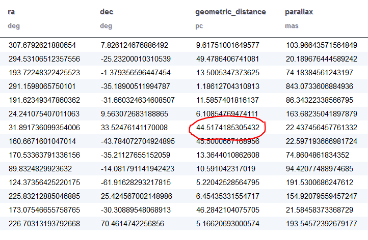
La plupart du temps, nous citons RA et dec en degrés: les RA vont de 0 à 360 degrés et les Dec tombent de -90 à +90 degrés. Mais vous verrez parfois le RA et le diminuer pour une source listée. en six chiffres: RA heures, minutes et secondes et déc degrés, minutes et secondes. Voici un outil pratique pour convertir la notation en heures, minutes et secondes en notation en degrés. (notation décimale et sexadécimale comme sur les GPS)

Dans ce flipbook, il y a des “dipôles” partout! Qu’est-ce que ça veut dire? Si vous voyez ce qui ressemble à plusieurs “dipôles” dans une image, cela signifie qu’il y avait un léger problème avec le pointage du télescope. Les étoiles ne bougeaient pas; le télescope l’a fait. Ce ne sont que des artefacts. Tous les artefacts stellaires ont tendance à danser – gardez simplement un œil sur ceux qui dansent différemment des autres. Les vrais dipôles (objets à déplacement lent) ressemblent à des dipôles dans les quatre images. Ils ressemblent un peu aux biscuits en noir et blanc, en particulier dans les première et dernière images (sauf que le glaçage blanc peut être bleu ou rouge).

null

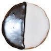
Est-ce un mover (objet qui se déplace) ? Cela ressemble à un motionnaire, mais n’apparaît que dans deux des images. Idéalement, un vrai mover devrait apparaître dans toutes les images. Si un objet n’apparaît que sur trois, il peut s’agir simplement d’un problème de bruit aléatoire. Supposez donc qu’il s’agisse d’un vrai mover (et que l’équipe scientifique tranchera). Mais s’il n’apparaît que sur deux images, il s’agit probablement d’un fantôme (artefact) et non d’un mover.

Que dois-je faire si je pense avoir découvert quelque chose? Tout d’abord, assurez-vous de le marquer dans chaque image avec l’outil de marquage. Ensuite, faites un commentaire sur sa page TALK en utilisant le #mover ou #dipole hashtag avec une description de l’endroit où trouver l’objet. Cela indique aux autres où regarder dans l’image (par exemple, “. #dipole rose pâle, coin supérieur gauche, RA 210.98, dec -22.53 “). Ensuite, vous voudrez vérifier s’il a déjà été publié dans la littérature astronomique à l’aide des outils décrits ci-dessous. Si vous trouvez un mover ou un dipôle n’est pas répertorié dans SIMBAD, s’il vous plait remplissez le formulaire! Si vous ne remplissez pas le formulaire, nous en apprendrons quand même sur votre découverte grâce à votre outil de marquage, mais il faudra peut-être plus de temps pour le trouver et le rechercher.

J’ai fait 100 classements! Pourquoi est-ce que je n’ai encore rien trouvé? Merci d’avoir fait toutes ces classifications ! En moyenne, il faut compter environ 60 classifications pour repérer un objet connu à mouvement propre correct. Bien sûr, ce ne sont que les objets que nous connaissons déjà; découvrir quelque chose de nouveau demandera un réel dévouement. Mais si vous avez fait 100 classifications et n’avez pas repéré de dipôles ou de déménageurs, vous allez peut-être trop vite. Prenez votre temps, regardez chacun des artefacts pour voir s’il danse différemment des autres, et assurez-vous que la luminosité de votre moniteur est augmentée au maximum. Il peut être utile de diviser mentalement les images en quatre quadrants et de ne regarder qu’un quadrant à la fois pendant la lecture de l’animation. Et rappelez-vous, même si vous ne trouvez rien, vos classifications sont toujours utiles; ils nous parlent de la fréquence ou de la rareté des nains bruns et de la manière de réduire les futures recherches de la Planète Neuf.

Comment utiliser SIMBAD? SIMBAD (ensemble d’identifications, de mesures et de bibliographie pour les données astronomiques) est une base de données pratique d’objets astronomiques utilisés par les astronomes professionnels et un outil crucial pour Backyard Worlds: Planet 9. Cet article de blog explique en détail comment l’utiliser pour vérifier si un objet que vous avez trouvé est déjà connu ou s’il s’agit d’une nouvelle découverte. Voici une explication abrégée.

Une fois que vous avez utilisé les chiffres sur le côté et le bas de chaque image pour estimer le RA et le déclic de votre objet préféré, vous pouvez interroger SIMBAD à cet emplacement pour voir s’il contient la liste des objets astronomiques connus. Par exemple, supposons que vous ayez repéré quelque chose d’intéressant à 277,68 degrés, 27,545 degrés. Aller à La page de requête de coordonnées de SIMBAD et tapez “277.68 27.545” et appuyez sur Entrée. Notez que ces coordonnées sont équatoriales (FK4 ou ICRS) et non galactiques ou écliptiques. Nous vous recommandons de définir le rayon de recherche sur SIMBAD (ou VizieR) sur 1 minute d’arc. De plus, si vous frappez le “i” dans un cercle sur la page TALK d’un sujet, vous verrez un lien vers SIMBAD qui recherchera toute l’image pour trouver des objets astronomiques (il cherchera dans un rayon de 498 secondes d’arc à partir du centre du flipbook).

Si SIMBAD ne trouve qu’une source sur l’image que vous regardez, cela vous mènera directement à une page d’informations sur cette source. Sinon, SIMBAD vous montrera une liste d’objets astronomiques classés dans l’ordre de leur distance par rapport au centre du sous-subtile. Cliquez sur les liens pour en savoir plus sur les objets trouvés par SIMBAD !

SIMBAD utilise une longue liste de abréviations dans ses tables. Par exemple, PM * = étoile rapide, BD * = naine brune, BD? = candidat naine brune, WD * = naine blanche. Vous pouvez en apprendre plus sur SIMBAD grâce à ceci Guide de l’utilisateur.

L’une des fonctionnalités les plus utiles de SIMBAD est que, pour chaque objet du catalogue, il dresse une liste des documents écrits mentionnant cet objet. Faites défiler vers le bas et 3/4 vers le bas de la page, vous devriez voir “Références”. Vous pouvez cliquer sur “trier les références” et voir les titres des articles où votre objet préféré a été mentionné ou discuté, le cas échéant. Assurez-vous de les parcourir. Votre objet préféré peut déjà faire l’objet d’un vaste débat international – ou peut-être simplement joué un rôle de calibrateur ou de référence astrométrique.

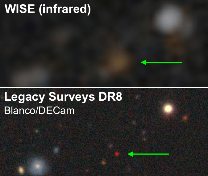
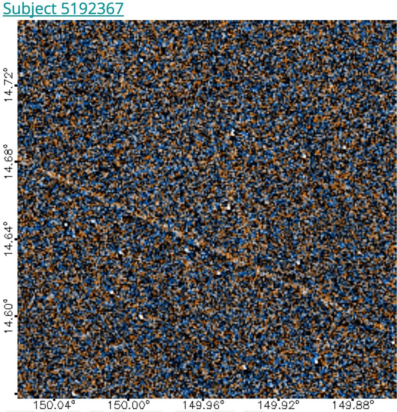
Comment utiliser le Finder Chart ? C’est un site qui montre la zone du ciel prise par différent télescopes et à différentes longueurs d’onde. Le lien est  NASA IRSA Finder Chart. Vous trouverez beaucoup plus d’images que ce que nous fournissons dans l’outil de clignotement. Contrairement aux images sur notre site Web, les images sur Finder Chart sont fixes, on ne peut pas détecter de mouvement. Ainsi, vous constaterez peut-être qu’un champ que vous pensiez presque vide est en fait assez peuplé de sources astronomiques !

Finder Chart vous montrera des images dans plusieurs bandes différentes: optique, infrarouge et infrarouge moyen. Chacun aura été pris à une heure différente. Si votre objet préféré est extrêmement froid (comme un naine Y ou une planète), il est possible que vous ne le voyiez pas dans d’autres images que celles de WISE. Si l’objet est chaud (comme une étoile), vous pourrez le voir sur plusieurs décennies, de l’imagerie optique à l’infrarouge moyen. Lorsque vous ouvrez Finder Chart, vérifiez que vous regardez le même champ de vision que celui que vous examiniez sur notre site Web en vérifiant si les mêmes étoiles sont présentes. Ensuite, vérifiez soigneusement si vous pouvez identifier l’objet dans d’autres catalogues (DSS, SDSS, 2MASS, WISE). Vous pouvez vouloir noter sur TALK lequel de ces catalogues vous pouvez le voir. De plus, si votre objet est un moteur, et que vous pouvez le voir dans les images de plusieurs catalogues (comme 2MASS et WISE), voyez si vous pouvez voir l’objet passant d’une image de catalogue à la suivante. Notez les dates de chaque image et le nombre de pixels (ou mieux, d’arcs secondes) qu’elle a déplacés. La distance parcourue divisée par la différence de temps (en secondes d’arc par an) indique la vitesse tangentielle de l’objet, un nombre crucial.

Un amateur (Guillaume COLIN, le traducteur de ce tutoriel !) a fait une vidéo qui explique en image comment utiliser ce site.

Que sont les “tiles” et les “sub-tiles” (terme anglais pour “tuiles”)? Le catalogue unWise divise le ciel en 18 240 “tiles”. Nous avons divisé chacun de ces éléments en 64 “sub-tiles”, qui sont devenus les images que vous voyez en ligne ici. Oui, cela fait beaucoup de sub-tiles. Le numéro de sub-tile est le numéro “ID” qui apparaît lorsque vous cliquez sur le “i” dans un cercle sous chaque image.

Comment utiliser VizieR? Si vous ne trouvez pas ce que vous recherchez dans SIMBAD, vous pouvez utiliser VizieR qui liste de nombreux catalogues astronomiques – presque tous les catalogues publiés ! Vous trouverez Une introduction beaucoup plus approfondie à VizieR dans cet article de blog. Mais voici quelques conseils de base.

Tout d’abord, tapez le RA et le dec de votre objet préféré où il est écrit “Recherche par position”, sélectionnez une “dimension cible” de 1 minute d’argent et cliquez sur le bouton “Go”. Alternativement, lorsque vous frappez le “i” dans un cercle sur la page TALK du sujet, vous trouverez un lien vers une requête VizieR qui effectue une recherche dans un rayon de 498 secondes d’arc du centre de l’image.

À la différence de SIMBAD, VizieR vous offre BEAUCOUP de listes de sources, une pour chacun des nombreux catalogues recherchés. Chaque liste est en ordre de distance par rapport au lieu recherché (soit les coordonnées que vous avez estimées, soit le centre du sub-tile). Chaque catalogue dans lequel il effectue des recherches a ses propres mises au point et mises en garde particulières. Vous devrez peut-être lire un certain nombre de fois pour tirer le meilleur parti de cet outil puissant. Essayez de combiner les résultats de la requête pour trouver des références à “mouvement correct”, car vous êtes le plus susceptible d’avoir identifié une source en mouvement. Par exemple, vous pouvez rechercher dans la page les lettres “pm” et rechercher des objets dont le mouvement correct est supérieur à 100 mas / an ou plus. Vous verrez souvent “pmRA” pour un mouvement correct dans Right Ascenscion et pmDE pour un mouvement correct en déclinaison. Si vous trouvez quelque chose qui n’est pas dans VizieR, veuillez le signaler sur TALK avec le mot #notinvizier hashtag.

Remarque: si vous trouvez votre objet sur VizieR mais pas dans SIMBAD, veuillez le soumettre au formulaire  Think you’ve got One toute façon.

Remarque: ne faites pas confiance aux mouvements appropriés répertoriés dans le catalogue AllWISE sur VizieR. Ils sont systématiquement faussement élevés. 

Pourquoi certaines images de ce flipbook sont-elles noires ou partiellement noires? Il y avait quelques problèmes dans la mission WISE qui l’empêchaient temporairement de prendre des données, et il en résultait des parties du ciel où il n’y avait pas de données à certaines époques (c’est-à-dire des périodes). Par exemple, entre le 3 avril 2014 et le 9 avril 2014, l’ordinateur de l’engin spatial a cessé de fonctionner correctement et la mission a dû être mise en “mode sans échec” pendant que la commande au sol le réinitialisait.

Quels objets en mouvement ont déjà été découverts? Cette feuille de calcul répertorie 3036 objets connus avec des mouvements propres> 600 milliarcsecondes par an. Vous en rencontrerez probablement certains pendant que vous effectuez une recherche. Mais même cette longue liste ne couvre pas tous les dipôles ou movers possibles; vous pourrez voir des dipôles avec un mouvement propre inférieur à 200 milliarcsecondes par an. Dans tous les cas, assurez-vous de vérifiez directement sur SIMBAD si vous pensez avoir découvert quelque chose de nouveau avant de le signaler à l’aide du  formulaire.

null

Quelle est cette bande géante sur l’image? C’est probablement un pic de diffraction associé à l’image d’une étoile brillante, proche de l’image que vous regardez. Les pointes de diffraction sont causées par la lumière diffractée par la structure de support du miroir secondaire du télescope. Les pointes de diffraction sont la raison pour laquelle les gens dessinent traditionnellement des étoiles avec des pointes qui leur tirent dessus. Mais en réalité, les étoiles sont plus ou moins rondes; les pointes sont créées par des télescopes et parfois par nos yeux.

Quelle est la taille des images que je regarde? Chaque image est de 256 x 256 pixels et chaque pixel est de 2,75 secondes d’arc. Ainsi, les images mesurent 704 x 704 secondes d’arc ou, de manière équivalente, 11,73 x 11,73 minutes d’arc ou 0,195 par 0,195 degrés.

Que faire si je vois un “mover” ​​qui sort du bord de l’image? Tout d’abord, lisez le article de blog sur les mover rapides. Ensuite, si vous décidez que cet objet est toujours intéressant (c’est-à-dire que ce n’est pas un coup de rayon cosmique ou un autre type de bruit), vous pouvez faire peu de choses. Tout d’abord, marquez-le lors d’une conversation avec le hashtag #mover et #outofframe pour que les autres puissent la suivre. 

Ensuite, il y a un site qui peut vous donner le lien vers les sub-tiles adjacents à l’image. Il a été créé par un utilisateur du site Dan Caselden WISEVIEW et a son propre article dédié.

Une fois rentré les coordonnées du centre de l’image, une vue animée apparaît. L’info que vous cherchez est dans le bandeau à gauche “Nearest Zooniverse tile”. Cliquez sur un des ID et ça vous amènera à une autre sub-tile. A vous de repérer par les coordonnées si c’est celui adjacent !

Pourquoi les RA et dec de cette image sont-ils perturbés ? les données UNWISE sont stockées à l’aide d’un projection gnomonique, qui fonctionne très bien sur la majeure partie du ciel. Mais près des pôles nord et sud célestes, les lignes de RA et de Dec ne correspondent plus à des lignes droites sur nos images! Ainsi, bien que les étiquettes des axes restent techniquement correctes près des pôles, elles ne sont tout simplement pas utiles. Ce n’est vraiment qu’un problème à environ 1 degré d’un pôle (c’est-à-dire pour moins de 0,2% des images). Si vous avez la chance de trouver un objet intéressant dans l’une de ces régions près d’un pôle, vous devez utiliser FinderChart pour estimer les coordonnées de cet objet. Cliquez simplement sur le i dans un cercle sur la page de discussion et cliquez sur le lien Finderchart. Placez ensuite votre curseur sur l’emplacement correspondant à votre objet. Les coordonnées apparaissent en haut de l’écran FinderChart. Vous trouverez peut-être utile de cliquer sur le bouton “Lock by click” (Verrouiller au clic) pour que, lorsque vous cliquez sur un objet de l’image, les coordonnées de cet objet restent affichées même lorsque vous continuez de déplacer le curseur. Là encore, la vidéo explicative suivante peut vous aider

Combien de flipbooks faut-il classer? Nous avons plus d’un million de sujets à classer. Mais la plupart d’entre eux ne sont pas encore en ligne. Donc, ne vous fiez pas au numéro de complétude sur la page de destination du site; cela ne concerne que le lot de flipbook déjà en ligne.

null

Quand allons-nous commencer à entendre les résultats du projet?

Notre Page Résultats page contient des liens vers des publications et des articles de blog sur nos résultats. Pour obtenir les dernières mises à jour, suivez-nous sur Twitter @backyardworlds ou Facebook!

Questions générales sur l’astronomie 

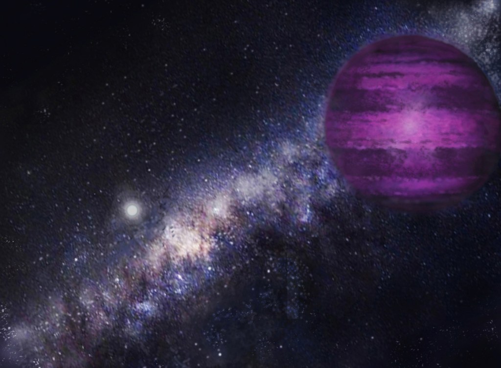
A quoi la planète 9 est-elle supposée ressembler ? Si elle existe, la planète neuf sera un mover peu mumineux et rapide. Le Field Guide contient une simulation de l’apparence possible. Contrairement aux naines brunes, la planète 9 est plus susceptible de se déplacer horizontalement dans nos flipbooks. En outre, contrairement aux naines brunes, il pourrait y avoir deux endroits où la planète 9 apparit car les images compilées ont été prises à différentes époques. Les deux apparitions seraient séparées d’environ 12 minutes d’arc, soit sur le même flipbook, soit à cheval sur deux.

La couleur de la planète neuf dépend de la quantité de méthane que contient son atmosphère. Selon les modèles de Fortney et al. En 2016, si la planète a une composition similaire à celle du Soleil, avec du méthane dans son atmosphère, elle sera plus brillante dans la bande WISE 2 et sera donc orange dans les flipbooks. Cette situation est plus probable si la planète neuf est plus massive que Neptune. Mais si le méthane a gelé hors de son atmosphère, ce qui semble probable si la planète ne compte que 10 masses terrestres, la planète sera plus lumineuse dans la bande WISE 1 et apparaîtra donc en bleu dans les flipbooks. Il est également possible que la planète soit trop petite et trop sombre pour être visible dans nos données…

Si vous pensez avoir trouvé la planète neuf, faites un commentaire sur sa page TALK en utilisant le bouton # Planet9 hashtag avec une description de l’endroit où trouver l’objet (par exemple, “rose pâle”) #mover, coin supérieur gauche, RA 210.98, dec -22.53 “). Vérifiez s’il existe un objet déjà publié dans la littérature astronomique à l’aide des outils décrits dans cette FAQ. Ensuite, si votre candidat à la planète neuf ne le fait pas se révèlent être répertoriés dans SIMBAD, s’il vous plait remplissez le formulaire!

null

Quelles sont les variables Mira? La plupart des objets les plus brillants que vous verrez à Backyard Worlds: Planet 9 sont des géantes rouges, qui palpitent souvent. Pour faire les images que vous voyez sur ce site, nous soustrayons une époque à une autre, afin que les étoiles variables se démarquent vraiment. Quoi qu’il en soit, si vous voyez un artefact stellaire énorme comme celui ci-dessus, c’est probablement un géant rouge qui palpite. Les variables de Mira sont une sorte de géant rouge palpitant. Ces étoiles géantes deviennent cent fois plus lumineuses et s’assombrissent de nouveau en l’espace d’environ un an.

À quoi ressemblent les naines brunes ? Les naines brunes, en revanche, sont connues pour être plus brillantes dans la bande WISE 2 (4,6 microns) que dans la bande WISE 1. Ils apparaissent donc en orange ou en blanc dans notre palette de couleurs. Ils peuvent être des “movers” ou des “dipôles”.

Qui d’autre est à la recherche de la planète neuf ? Plusieurs autres groupes recherchent Planet Nine. Dark Energy Survey utilise un télescope dédié à l’observatoire interaméricain Cerro Tololo. le Pan-STARRS enquêteutilise un télescope dédié sur le mont. Haleakala à Hawaii. Le télescope Subaru à Hawaii effectue également une recherche plus approfondie mais plus ciblée. Le SkyMapper Survey utilise un télescope dédié à l’observatoire de Siding Spring en Australie; Cette étude est la base pour un autre projet de Zoonivers appelé simplement “Planet 9”.

Toutes ces autres projets effectuent une recherche dans les longueurs d’onde visibles à l’aide de télescopes au sol, tandis que chez Backyard Worlds: Planet 9, nous examinons l’infrarouge à l’aide d’un télescope dans l’espace. Cela nous permet de chercher dans tout le ciel, plutôt que de nous limiter à un coin de ciel. Personne ne sait encore si Planet 9 sera plus lumineux aux longueurs d’onde infrarouges où nous travaillons ou aux longueurs d’onde visibles où les autres recherches fonctionnent. Il est donc logique de chercher dans les deux parties du spectre. Lisez Le blog d’Aaron Meisner pour en savoir plus.

Pourrait-il y avoir plus de planètes au-delà de la planète neuf? Il est possible qu’il y ait plus de planètes invisibles en orbite autour du Soleil, en plus de la planète neuf. Volk et Molhotra (2017) ont récemment suggéré qu’une dixième planète pourrait être responsable de la création d’une chaîne dans le plan de la ceinture de Kuiper. Cette petite planète serait probablement trop faible pour que nous puissions la détecter ici sur Backyard Worlds: Planet 9. D’autres planètes pourraient encore se cacher au-delà de l’orbite putative de la neuvième planète. Mais il n’y a pas encore de preuve particulière en faveur d’une onzième planète, comme la preuve dynamique que nous avons pour une neuvième planète.

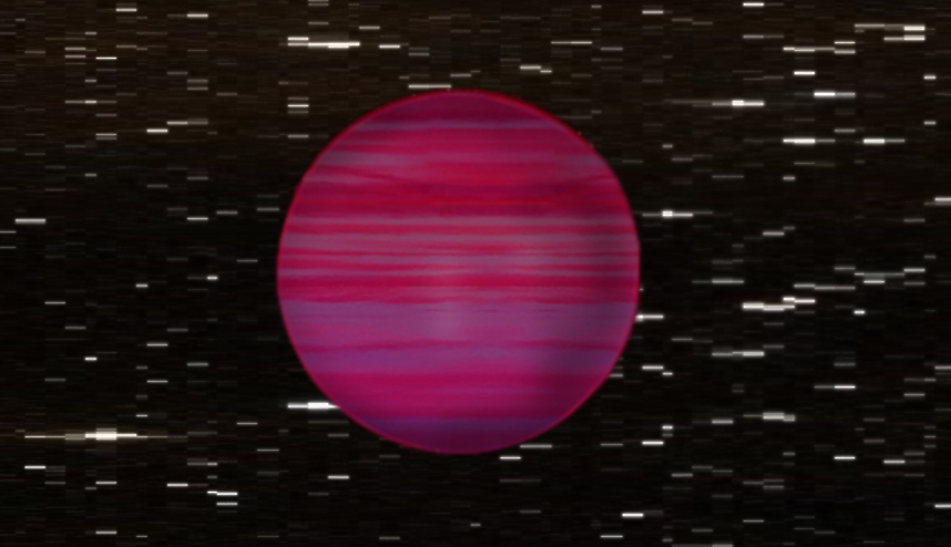
Pourquoi nous intéressons-nous aux naines brunes? Les naines brunes sont le lien entre la formation d’étoiles et la formation de planètes. Ils ont des caractéristiques physiques qui se chevauchent à la fois avec les étoiles et les planètes. En comptant leurs nombres et en déterminant leurs masses, nous pouvons apprendre comment se forment les étoiles, les planètes et les galaxies. Les naines brunes froides sont particulièrement pratiques car nous les utilisons comme analogues aux exoplanètes. Ils ont la même taille que Jupiter, et parfois la même température que Jupiter ou même la Terre, mais ils sont beaucoup plus faciles à étudier que les exoplanètes, car ils ne gravitent pas autour d’étoiles brillantes qui les submergeraient d’éblouissement. Par conséquent, nous pouvons obtenir des informations très détaillées sur leurs atmosphères, qui nous renseignent sur leur composition, leur rotation, les nuages, les tempêtes et même les propriétés magnétiques. Certains naines brunes ont même les planètes qui les orbitent. En travaillant avec vous sur ce projet de science citoyenne, nous espérons découvrir des naines brunes exotiques dotés de caractéristiques nuageuses qui nous aideront à comprendre la diversité des atmosphères présentes dans les exoplanètes. Pour en savoir plus, lisez Le blog de Jackie Faherty.

Combien de naines brunes attendons-nous à trouver? Nous avons Une bonne idée du nombre d’étoiles et de naines brunes qui se trouvent à proximité, avec des types spectraux de L2 et plus anciens (plus chauds), mais la plupart d’entre eux ont probablement déjà été découverts. Les derniers types (plus froids) restent mystérieux. L’un de nos principaux objectifs chez Backyard Worlds: Planet 9 est de résoudre le problème de la fréquence des naines brunes les plus froides !

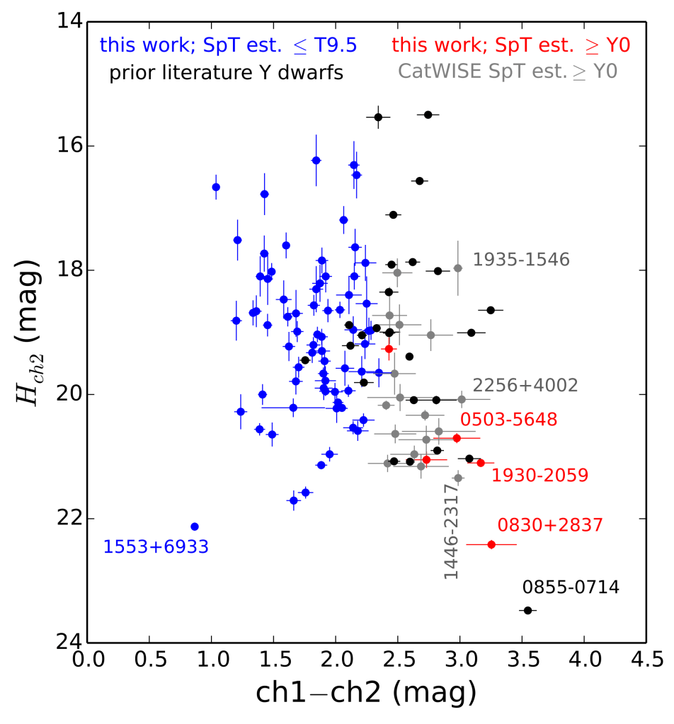
Retour en 2012, Kirkpatrick et al.2012 Selon les estimations de, il y aurait environ 5 naines brunes de types T6-T8.5 et au moins 6 des types T9 et ultérieurs (plus froides) à moins de 7 parsecs du Soleil. Mais alors Luhman (2014) a découvert un nouvel objet appelé WISE J085510.83-071442.5 qui a battu le record du naine brune la plus froide et contraint les utilisateurs à refaire leurs estimations. Depuis, Zapatero Osorio et al. 2016 a estimé qu’il devrait y avoir entre 15 et 60 naines Y2 à moins de 7 parsecs du Soleil. Pendant ce temps, Yates et al. En 2016, nous prévoyons qu’il y a environ 3 naines Y avec des types compris entre Y0 et Y0.5 dans le Soleil, sur environ 10, et seulement 1 avec un type spectral plus récent (plus froid) (c’est-à-dire Y1, Y2, etc.). Comme vous pouvez le constater, le large éventail de ces estimations s’explique par le fait qu’il s’agit d’extrapolations à partir d’une liste ne contenant que quelques objets.

Combien de naines brunes sont déjà connus? Milliers. DwarfArchives.org répertorie actuellement 1281 naines brunes (en date de 2012). Cependant, seulement vingt-quatre naines brunes connues sont “froides” (température ambiante) naines Y, et seulement trois sont situés à moins de 10 années-lumière du Soleil. Nous espérons trouver plus de ces objets rares et proches.

Que sont M dwarfs (naines), L dwarfs, T dwarfs and Y dwarfs ? Comme les étoiles, les naines brunes sont classées en fonction des raies d’absorption trouvées dans leur spectre, qui sont des indicateurs de leurs températures de surface. Les naines M sont environ 3500-2100 K, Les naines L sont 2100-1300K, les naines T sont 1300 à environ 600 K, et  on estime que les naines Y sont plus froid que 600 K. Comme les naines brunes sont tous de la même taille physique, le plus bas est la température, moins lumineux elle est. Les “types” de naines brunes sont une continuation de la séquence des types stellaires; la liste complète des types va de O, B, A, F, G, K, M, L, T, Y. Chaque type a des sous-types, indiqués par des chiffres, qui décrivent des variations plus subtiles de la température. Par exemple, une naine T6 est plus froid qu’une naine T3. Les étoiles et les naines brunes peuvent être des naines M; Les naines brunes ne deviennent généralement pas plus chaudes qu’environ M6. Voici un pratique article de synthèse d’Adam Burgasser avec plus d’informations.

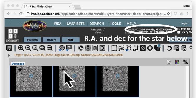
Quel est la naine brune connue le plus proche? Une paire de nains bruns appelés Luhman 16 ou WISE 1049-5319 est situé à 6,52 années-lumière (1,99 parsecs) du Soleil; ce sont les nains bruns connus les plus proches. Peut-être en découvrirez-vous un qui est encore plus proche ! Ce diagramme (crédit: NASA / Penn State University) montre l’emplacement des étoiles et des naines brunes les plus proches.

null

Quelle est l’étoile la plus proche du soleil? Proxima Centauri est l’étoile connue la plus proche du Soleil. Cela semble être le membre le plus faible d’un système à trois étoiles, appelé Alpha Centauri, et donc aussi appelé Alpha Centauri C. Il est étrange que l’étoile connue la plus proche soit plus proche que le naine brune connu le plus proche? N’y aurait-t-il pas une naine brune plus proche encore ?

Pouvons-nous voir des planètes naines dans la ceinture de Kuiper ou d’autres objets de la ceinture de Kuiper dans ces images? Non, ils sont trop faibles à ces longueurs d’onde.

Que signifie MJD? MJD signifie Date julienne modifiée, (Modified Julian date) nombre de jours écoulés depuis le 17 novembre 1858 à minuit. Chaque image astronomique de ce site Internet est horodatée avec une date julienne modifiée indiquant à quel moment elle a été prise.


The Crystal Ball White Dwarf

Today is a big day at Backyard Worlds: Planet 9!  We’re celebrating our 2nd anniversary, our reboot, and announcing our second paper, published in the Astrophysical Journal letters.   (You can read it here for free.) It’s about a unique white dwarf that’s an analog for the solar system three billion years from now; the oldest white dwarf known to host a dusty disk, the likely remains of a planetary system.   Check out this guest blog post by our own Melina Thévenot, who explains how she discovered this record-breaking object, which provides such a chilling glimpse into the future.

Melina Thevenot
Melina Thévenot, the citizen scientist at Backyard Worlds: Planet 9 who discovered the infrared excess from white dwarf LSPM J0207+3331.

Hi everyone. I am Melina Thévenot, a volunteer of the Backyard Worlds: Planet 9 project from Germany. Here I want to tell you a bit about how I discovered an unusual white dwarf and how the researchers uncovered that it is not only unusual, but also cool.

How did I discover the white dwarf LSPM J0207+3331?

As a volunteer of the Backyard Worlds: planet 9 project, I spent a lot of time searching for brown dwarfs. The Gaia Data release 2 was my favorite survey for the search of brown dwarfs. I uncovered probably several hundred new brown dwarf candidates that move in wiseview with the help of three other volunteers: Katharina Doll, Hugo Durantini Luca and Peter Jalowiczor. 

While improving my search I noticed something about brown dwarfs in the Gaia catalog: some good sources don’t have color information in Gaia DR2. This is a problem, because I relied on a color-cut. To check if I missed any good T-dwarf, I decided to use Allwise to find sources with high infrared excess and the high parallax measurement in Gaia DR2. In the resulting list I could find fake sources that did not move in wiseview, T-dwarfs (distance 5 to 10 parsec) and one source that does not belong in this list.

I don’t remember where I saved the original list, but it probably looked like this:

list

The object in the red circle has a distance of 44 parsec. Gaia should not detect a T-dwarf at this distance.

Is it another fake source? I could have ignored it. I am glad I checked the movement.

Wiseview link: http://byw.tools/wiseview#ra=31.891736099354006&dec=33.52476141170008&size=60&band=3&speed=295&trimbright=98.88&linear=0.845&color=gray&mode=percent&coadd_mode=pre-post&zoom=17&border=0

As you can see: Compared to the background objects it is moving and in PanSTARRS you can see a blue source.

This source is LSPM J0207+3331. At this time I still had no clue what it could be. I did need some days to think about it. After checking the position in a HR-diagram I knew that it was a white dwarf with large infrared excess (Allwise w1-w2≃1). I guessed that this excess comes from a circumstellar disk. Time to loop in some other volunteers, who are advanced users of Disk Detective. Katharina Doll told me that the source looks good and she confirmed that it was possible for a white dwarf to have a disk, something I did not know until she told me. We decided to contact Marc Kuchner and soon John Debes joined the discussion.

Observation with Keck

John Debes told us this white dwarf is cold, in fact it was 1000 Kelvin cooler than any known white dwarf with an infrared excess. So the researchers decided to observe it with APO. But the dome was closed because of bad weather. Soon the white dwarf was observed with Keck! The telescope with the largest mirror on this planet!

I watched closely how things developed. I made a timeline:

Date
2018-10-17 Discovery of LSPM J0207+3331 (still no clue what it could be)
2018-10-19 Sending LSPM J0207+3331 to the researchers
2018-10-20 Bad weather at APO
2018-10-27 LSPM J0207+3331 is being observed with Keck (Adam Burgasser observed it for us – THANK YOU!!)
2018-12-01 Paper is submitted to ApJ Letters
2019-02-02 Paper is accepted


A 3 Gyr White Dwarf with Warm Dust

Let’s talk about the paper. Des Pudels Kern. (German Saying, “The core of the poodle” meaning the main point)

What is a white dwarf? Our sun will develop into a red giant billion of years in the future. The red giant will lose the outer layers in a Planetary Nebula. The core that is left is a hot white dwarf and it will gradually cool and become fainter.

The process is very violent and “loosing the outer layers” is nothing else than burning the orbiting planets in strong solar winds. But not everything will perish. White dwarfs have a leftover stellar system with asteroids, comets and planets. If an asteroid or comet comes too close to the white dwarf, it can be torn apart by the tidal forces caused by the gravity of the white dwarf and the material settles down in a disk around the white dwarf.

figure 1 of the paper

In figure 1 of the paper you can see a blue line. This is how the Spectral Energy Distribution (SED) of the white dwarf should look like without a disk. The gray lines are the spectra from Keck NIRES and the black squares are the photometry from different surveys. You can see how the spectra and the photometry are somehow taking off to the right side. This blog post from Disk Detective explains what a SED is and how a SED looks like for star+disk. It might help you interpret this figure. 

Models that try to describe disks around white dwarfs predict that young white dwarfs are more likely to develop a disk. It is therefore surprising that a 3 Gigayear (3 Billion years old) white dwarf has a disk. Is LSPM J0207+3331 special or are the models about the formation of disks around white dwarfs not accurate enough? Future searches for similar white dwarfs might shine light on this mystery.

But this is not where the story of this white dwarf ends. The disk around LSPM J0207+3331 is not a simple disk, but it consists of two components: an outer colder ring with a temperature of 480 Kelvin and an inner ring with a temperature between 550-1400 Kelvin. The white dwarf has an temperature of 6120 Kelvin and a mass of 0.69 solar masses. The outer ring might have formed from a small asteroid that was disrupted by the tidal forces in the recent history of the system. This is the first time such a system was observed.

In the future, researchers will observe this white dwarf again and obtain more data, which might tell more about this system. An optical spectrum, for example, might tell us if any material from the disk is falling into the atmosphere of the white dwarf, and what that material is made of.

I am very proud to be part of this discovery and hope you enjoyed reading this blog post.

The Reboot Is Here!

Team,

As you may know, the WISE mission has continued to scan the sky during the last few years—collecting more images for us to search.   So we’ve started uploading new batches of subjects for you to classify that incorporate new WISE data.

These new subjects are improved in at least four ways:

  1. They include two entire new years of data, so they cover a 50% longer time span. That means movers move farther and dipoles look brighter.
  2. The Poisson noise and the amplifier noise (the stripes) are reduced by at least 41%, sometimes by a factor of up to 10 in regions near the ecliptic poles.
  3. All the images have been realigned, so stationary stars subtract out better.  Some of the artifacts and ghosts have been averaged away in the process too.
  4. Planet 9 and other solar system planets no longer hop and jump.  They are simply ordinary dipoles or movers.  (If they exist.)

We’ve also taken this opportunity to fix some of the broken links in the metadata and add some handy new ones, like links to WiseView  and to WISE images on LegacySurveys. Now, it might not be obvious immediately that you’re looking at a reboot image; they might look at first glance to be just as noisy as the pre-reboot images you’re used to.  That’s because we cranked up the gain to match the noise reduction!  So they images look just as noisy, but now the objects you’re looking for will be at least 41% brighter.  You can always tell you’re looking at a reboot subject if the metadata includes links to WiseView and LegacySurveys and doesn’t say anything about the motion of planet nine.

Now, there’s something important to be aware of when you’re using the reboot data. There are still four frames like you’re used to.  But now the biggest time interval is between the first and second frames.   Previously, dipoles tended to flip sides between frames 2 and 3.  But now, the dipoles will tend to flip between frames 1 and 2.  We’ll be updating the tutorials and field guide to illustrate this change (and if you have any nice examples that you think we ought to show, please bring them to our attention).

RebootExample_animation
Nearby Y dwarf WISE 0855 before and after the reboot. The brown dwarf (moving red dot, upper left) moves farther and faster in the reboot flipbook (right), and the stars dance less.  The biggest time step, when you see the red dot move the farthest, is between frames 1 and 2 in the reboot flipbook,

Unfortunately, each new subject will have its own new TALK page, even if it covers the same region os sky as an older subject.  But there will often be a link in the metadata to the old TALK page (if it exists).  There will also be links in the metadata to the old TALK pages of the adjacent subtiles, to help you track a dipole or mover that seems to go off the edge of the image.

We will be re-uploading the whole sky bit by bit over the next few months.  This is a big project.  But we’re starting with a sector that we have not yet looked at before so there there should be some nice new things to discover right away.

Thanks for all the hard work you put in so far—you made it through about 2/3 of the sky once already!   Now we’re gonna start fresh and kick it up a notch.  Have fun!

Marc Kuchner


42 Confirmed Brown Dwarfs and Counting

Hey everybody!   Thanks to your efforts, we’re now up to 879 brown dwarf candidates.  Wow.  We’ve been following up your discoveries as fast as we can, getting spectra to determine their spectral types and distances, test for membership in moving groups, and look for unusual features. For the coolest objects, we’ve also been working on taking new images.  Here’s a little update on all this follow-up work.

First of all, we have a big stack of new spectra. Jackie Faherty confirmed 17 of our brown dwarf candidates with the ARCoIRIS spectrograph on the Blanco 4m telescope in Chile, and Jonathan Gagné, Jackie Faherty and Michaela Allen observed another batch of 8 targets with the SpeX spectrograph on NASA’s Infrared Telescope Facility (IRTF).  Of those 8 we observed with IRTF, 6 are brown dwarfs. The other two are late Ms; one has a co-mover (spotted by Tadeas Cernohous) and the other has an unusual J band flux that threw off our initial spectral type estimate.

Picture of Michaela Allen’s desk at NASA Goddard Space Flight Center while she was observing our brown dwarf candidates remotely with the IRTF telescope.

That’s right, Michaela, our TALK moderator, is now participating in observing runs! Michaela is spending her summer as a NASA intern here at Goddard Space Flight Center in exotic Greenbelt, Maryland.  She’s working on our Gemini data, and looking through the long long list of moving objects you have found that did not appear, at first glance, to be brown dwarfs.  You can follow her on Twitter @sasstronaut42 to find out more about how her summer is going, and you’ll hear more about her work later on.

Thanks to Jackie, Jonathan and Michaela’s hard work, I can now say that we have confirmed a total of 42 brown dwarfs.  These confirmed objects include 10 L dwarfs and 32 T dwarfs.  Of these, fourteen are closer than 20 parsecs, and four are closer than 15 parsecs. Congrats to Nikolaj Stevnbak Andersen, Dan Caselden, Guillaume Colin, Sam Goodman,  and Melina Thevenot, whose TYGO form submissions were observed with ARCOIRIS and confirmed to be brown dwarfs!   And congrats to Nikolaj Stevnbak Andersen, Dan Caselden, Tadeas Cernohous and Guillaume Colin, whose TYGO submissions were observed with IRTF and confirmed to brown dwarfs!  I believe those are Nikolaj’s, Tadeas’s and Melina’s first brown dwarf discoveries.

The “seeing” at IRTF was only about 0.8 arcseconds, which is poor for that site, and there were thin cirrus clouds. So we were only able to take decent spectra of objects brighter than about 16th magnitude in J band.  So this run was a bit disappointing.  But just today we learned that we won four more nights on IRTF this fall! 

In fact, here’s a summary of our follow-up program so far—where we’ve been an where we’re going.    The “R” value is the spectral resolution of the spectrograph we’re using. R = the central wavelength of the spectrum divided by the smallest difference in wavelengths the spectrograph can distinguish.   So larger R means finer resolution.  But finer resolution comes at a cost; you need to collect more light to begin with if you’re going to spread it out more by wavelength.

Table 1. Status of our follow-up observing program.
Gemini-North/NIRI Fast Turnaround J/K band imaging 9.2 hours, 16 targets Images of 16 targets obtained
Magellan/FIRE Prism R~450 17 targets Spectra of 17 targets obtained
Apache Point Observatory (APO)/Triplespec R~3500 1 night Bad weather, spectra of 2 targets obtained
Blanco 4 m/ARCoIRIS R~3500 2 nights Spectra of 17 BDs obtained (see above!)
Magellan/FIRE Echelle R~7000 1 target Spectrum of 1 target obtained 2/3/18, RV measured
Infrared Telescope Facility (IRTF)/SpeX R~150 2 nights, 20 targets 1 night weathered out, spectra of 8 targets obtained during second night (see above!)
HST/WFC3 F125W/F105W imaging 5 orbits, 5 targets Awarded 5 orbits
Mont Mégantic/CPAPIR J-band imaging 8.5 hours, 60 targets


Awarded time to observe 60 targets. Images of 12 obtained May 2018
Magellan/FIRE Prism


R~450 1 night, 20 targets Awarded 1 night in 2018B
Keck/NIRES


R~2700


1.5 nights, 10 targets Awarded 1.5 nights in 2018B
Spitzer


3.6 and 4.5 micron imaging 26.8 hours, 65 targets Awarded 26.8 hours
Infrared Telescope Facility (IRTF)/SpeX R~150 4 nights, 40 targets Awarded 4 nights in 2018B
Gemini-South/Flamingos 2 R~600 13.7 hours, 27 targets Proposal Submitted, Pending
Magellan/FourStar J-band imaging 1 night, 8 targets Proposal Submitted, Pending
Gemini-North/GNIRS R~11,800 9.4 hours, 5 targets Proposal Submitted, Pending

Keep up the amazing work!  And stay tuned for more cool discoveries!!

Marc