Backyard Worlds: Planet 9

Guest Blog Post by Peter Jalowiczor

(One of our volunteers, Peter Jalowiczor, gave a talk about Backyard Worlds: Planet 9 at his own astronomy club. Today’s informative blog post is his report about the experience. Did you know that brown dwarfs get smaller the more massive they are? Read on. -Marc)

I had the pleasure to give a talk at one of the UK’s leading Astronomical Societies: the MSAS (the Mexborough and Swinton Astronomical Society). The society is situated ~20 km from Sheffield (pop, 570,000) in England and was founded in 1978. Every Thursday evening is a great social occasion centred on a lecture. At least once a month, some academic visits the society to present on an aspect of Astronomy. Academics really enjoy visiting and describe this place as an Aladdin’s cave as may be seen by some of the photos!

2018 146 MSAS Presentation — The first slide of Peter’s presentation.

The evening was divided-up into two parts consisting of two completely different presentations. One sent by Marc specially for the occasion and the other prepared weeks in advance by myself. They turned out to complement each other perfectly (thank you Marc!). You’re welcome, Peter! -Marc

The First Presentation

I started with an introduction to the Science team and the important fact that Planet Nine is presumed to exist. It is estimated to be around 10 Earth masses, on an elliptical orbit, averaging a=700 AU because of visible disruption in the orbits of detached Kuiper Belt Objects. Next, the nearest neighbours to the Sun were discussed with examples of these BD systems and the prizes of participating in BYW:P9 included discovering such objects.

The flipbook was introduced followed by examples of what to mark and what not to mark: the submissions procedure. How this would be related to the Astronomical software/ procedures described in the second presentation blended both presentations ideally.

The successes of BYW:P9 include the discovery of a T Dwarf in the first few days of the project!

2018 166 MSAS Presentation — Members of the Mexborough and Swinton Astronomical Society, enjoying Peter’s presentation, and thinking up tough questions (see below).

The Second Presentation

I started with a comprehensive description of brown dwarfs, with the three main categories and their associated spectral classes; this culminated in a review of the mass-radius relationship from solar-type stars to the terrestrial planets (G. Chabrier et. al., 2008). A chart demonstrated the decrease (compression) of BD radii with mass before the critical mass is reached as a BD turns into a star. After this point the radius increases dramatically. The positions of L, T and Y objects and sub-BD objects was discussed down to Jovian mass.

MassRadiusdiagram — Mass-radius diagram for planet, brown dwarfs and low-mass stars, from Fortney, Baraffe and Militzer 2014. More massive brown dwarfs are slightly smaller than less massive ones.

Second, I a gave detailed description of the 2MASS project and the WISE mission, the wavebands in which the detectors operated and the positions of the IR bands on the electromagnetic spectrum. 2MASS: j=1.235um, h=1.662um, k=2.159um. WISE: W1=3.4um, W2=4.6um, W3= 12um, W4=22um. I showed that WISE goes much deeper than 2MASS into the Mid-Infrared.

Third, I gave a complete overview of the astronomical tools used: the Backyard Worlds: Planet 9 flipbook, which is at the heart of the project, SIMBAD, VizieR, IRSA Finderchart and BYE Tools (Wiseview).

Fourth, I showed a home video of how everything comes together.

Fifth, I described the project’s results by showing a presentation of the spreadsheet that has been built-up. I described how the photometry of 2MASS and WISE come into this, i.e., W1-W2, J-W2 and how these differences can be used to constrain the spectral types of objects. I referred to photometric Brown Dwarf classification charts from Skrzypek, N., et al.,

I showed clips from Backyard Worlds: Planet 9 Hangouts to demonstrate the international calibre of this project, which put on a completely different light on everything.

Illustration of the spectral coverage provided by the DustPedia database, showing filter response functions of all bands for which we present data. As can be seen, the data we employ effectively provides complete sampling of over five orders of magnitude in wavelength. Response functions of the bands for which we present both imagery and aperture-matched photometry are traced with solid lines. Bands for which we present supplementary external photometry are traced with dashed lines. Bands for which we present imagery only are traced with dotted lines. — The spectral bands used by 10 different survey telescopes. 2MASS (blue) and WISE (leftmost greeen) are the surveys we use in Backyard Worlds: Planet 9.

And finally!

The principle aims of the project are to discover Brown Dwarfs and Planet Nine. Red Dwarfs are a secondary target and are being catalogued.
Volunteers are encouraged to distinguish real celestial objects from image artefacts in data from NASA’s WISE mission
roughly 5 million classifications of images from NASA’s WISE telescope.
432 objects of interest for the follow up campaign, mostly newly discovered BD candidates. We now have more than 500! -Marc
Planet Nine has remained elusive, as have Planet X and Tyche (instruments are sensitive to gas giants out to about 50,000 astronomical units from the Sun).

—Peter Jalowiczor

There was also Question and Answer Session at the end of the lecture. I’ve attempted to answer some of the questions. –Marc

Q: What causes the ‘ghosts’/artefacts in the images?

A: Though the optics in the WISE telescope are first rate, they are not perfect; some black surfaces are not perfectly black, and some transparent optics are partly reflective. As a result, the light from particularly bright stars can create secondary images from bouncing around more than, ideally, it should. Those appear as artifacts and ghosts. –Marc

Q: The candidates submissions procedure. If it is listed in a Red Dwarf catalog. There seemed to be contradiction in what I said and what seemed to implied by the project. (e.g. I don’t submit a candidate if it is listed in a Red Dwarf catalog in VizieR). Whereas there could be objects listed in Red Dwarf catalogues that are misclassified? Should such objects be submitted or not? It would save time for the user.

A: The rule is: if it’s moving and it’s not in SIMBAD (and not a ghost or star or other artifact), please submit it to the Think-You’ve-Got-One form. Sorry for the confusion! -Marc

Q: Brown Dwarfs or Brown Dwarves? One member picked-up on this after I used this (I was using Brown Dwarfs). It turns out that Dwarfs is American English and Dwarves is British English. I was ‘instructed’ to write properly!

A: I’m no expert on British English, but perhaps you could consult with the Extrasolar Planets and Brown Dwarfs group at the University of Hertfordshire.

Thank you, Peter, for being such a compelling ambassador for Backyard Worlds: Planet 9, and for composing this delightful blog post. –Marc

BYWP9 Peter Jalowiczor — Pete at his computer working on Backyard Worlds: Planet 9.

We Love You! And Happy Anniversary!

Team,

This Thursday, February 15, marks the one year anniversary of the launch of Backyard Worlds: Planet 9. What a year it has been! Let me attempt to sum up where we are, scientifically. It’s hard not to stop and gasp in awe at all you’ve accomplished.

AnniversaryImageBYP9 For starters, you have performed 4.775 million classifications of images from NASA’s WISE telescope. (The backyardworlds.org site only shows classification numbers for the current batch of subjects–you have done about 322,000 classifications of those.) You have also submitted more than 20,000 objects on the Think-You’ve-Got-One form. All this hard work has yielded 432 objects of interest for our follow up campaign, mostly newly discovered brown dwarf candidates.

Because of these objects–and your interest in this work–seem so promising, this fall we were awarded a grant from NASA ‘s Astrophysics Data Analysis Program that will keep us working on the project with you into the year 2020.

Mauna Kea Observatory — In two weeks, we’re headed to NASA’s Infrared Telescope Facility to follow up more brown dwarf candidates.

Soon afterward, we were awarded five nights of telescope time on NASA’s Infrared Telescope Facility, Apache Point Observatory, and the Blanco 4-meter. That should be enough to follow up about 100 of your discoveries. We have only had a chance to use one of these nights so far–and it was cloudy! Yet, thanks to donations of observing time from other projects, we have managed to collect spectra for 20 brown dwarf candidates (Thank you, Jonathan Gagne and Katelyn Allers!). These spectra show that we have discovered 17 new brown dwarfs. Their spectral types and distances, in units of parsecs (pc) are all listed at the bottom of this post.
Only three of the objects we have followed up so far turned out not to be brown dwarfs. Two of these objects (first reported by Sam Goodman, Dan Caselden, and Guillaume Colin) are newly discovered cool subdwarfs, a rare class of metal-poor stars. The one other is an unknown object that’s not really moving, though it might be time variable. So I’d say our batting average is 95% (I supposed that would be .950 if it were an actual batting average).Congratulations to the citizen scientists who spotted these 17 brown dwarfs! They are: Dan Caselden, Rosa Castro, Guillaume Colin, Sam Deen, Sam Goodman, Bob Fletcher, Les Hamlet, Jörg Schümann, Khasan Mokaev, and Tamara Stajic.

As you can see from the list, we’re getting close to our dream of finding Y dwarfs. The newest batch of follow-up spectra contained a T9, our coldest brown dwarf find yet, just one subclass warmer than Y0. And we have 38 Y dwarf candidates that we have yet to get spectra of! These take some extra work to follow-up because they are so faint, but we will be working our way down that list over the next year. Note that there are only about 25 known Y dwarfs so far, found by other surveys. So even if only half of our candidates pan out, we will have made a big difference to the field.

We haven’t yet found any brown dwarfs closer than Proxima Centauri (1.3) parsecs or Luhman 16 (2.0 parsecs). But they might well be out there, waiting for us. Three of our brown dwarf discoveries are closer than 20 parsecs, so they will have an impact on statistical studies of brown dwarf populations. Our list of candidates contains 25 more that are closer than 20 parsecs, including five closer than 15 parsecs.

We may have already found some young moving group members–brown dwarfs that are young, with relatively well-constrained ages, that could potentially be rogue planets. We have taken spectra now of two objects that seemed likely to be moving group members. No luck yet, but one object was a very near miss. Our initial estimates showed a > 90% probability for membership in the AB Doradus moving group. Then, when Jonathan Gagne observed it with the FIRE spectrograph on Magellan, he saw a spectrum that closely resembles that of GU Psc b, a planetary-mass T dwarf in that AB Doradus. So the next night, Jonathan took an might higher resolution spectrum of this object to measure its radial velocity, i.e., how fast it is moving in the direction along our line of sight. Alas, it turned out that the radial velocity was is not consistent with the AB Doradus moving group. But among our candidates are 20 more possible moving group members we haven’t yet been able to check.

Most stars in the galaxy come in multiple systems–and brown dwarfs often have companions as well. So we’ve been searching the literature, with help from our citizen scientists, to check for companions to our brown dwarf candidates. We spotted five such likely pairs so far (though one of the companions orbits around a candidate subdwarf, not a brown dwarf). Finding a companion like this around a brown often allows you to constrain the brown dwarf’s age and mass. So we’ve prioritized these for our follow-up campaign. Congratulations to Tadeáš Cernohous, Jörg Schümann and Andy Fischer for finding the comovers.

When a brown dwarf has a near infrared “color” that is unusual for its type, it can inform us. Brown dwarfs that are redder than average are often younger; blue brown dwarfs may be metal poor. About 19 of our brown dwarf candidates have stood out to us as having unusual colors. Plus, the spectra we have taken turned up two unusually red objects, and three more that seem notably blue.

Planet Nine has so far remained elusive, as have Planet X and Tyche (we are sensitive to gas giants out to about 50,000 astronomical units from the Sun). But we’ve acquired some useful search experience that we’re going to put to use when we reboot the site this spring (see below). Also…nobody else has found any new planets beyond Neptune yet either.

So what’s next? Well, we think there are probably roughly 800 more brown dwarfs to find in the data that’s online so far. And clearly our follow-up campaign is just beginning.

But that’s not all. As we’ve mentioned, WISE has continued to take new data since the project launched, and already 2 more years of images have been recorded, beyond what’s online at backyardworlds.org! We’re working on adding those to the flipbooks, to help you disentangle dipoles from stars and movers from cosmic rays. They should make our search for new planets in the solar system much easier too, allowing us to process the data in a way that avoids the mess of different hopping and jumping patterns. In the meantime, we’re working on more telescope proposals to follow-up the objects you discovered already. So keep searching, and stay tuned for a reboot of the whole site in the next few months! And thank you for a thrilling, inspiring first year.

Happy Valentine’s Day!

With love from Marc Kuchner and the Backyard Worlds: Planet 9 Science Team

T3	16.8 pc
T9	17.1 pc
T3.5	17.6 pc
T8	19.0 pc
T7	21.6 pc
T6.5	21.7 pc
T8	22.5 pc
T5	25.0 pc
T4	29.1 pc
T6	30.2 pc
T5.5	33.7 pc
L9	34.0 pc
L9.5	37.0 pc
T0	40.6 pc
T5	45.7 pc
L2	48.4 pc
L5	64.1 pc

This table lists our brown dwarf discoveries so far.

Snow White and the Seven New Confirmed Brown Dwarfs

It is now winter here in the northern hemisphere, and we’re expecting snow on Friday in Washington, DC. But fear of snow doesn’t stop us from going observing…and observing we have been! Jonathan Gagne returned from his last trip to the telescope with spectra of nine of our brown dwarf candidates—and seven of them are now bonafide brown dwarfs. That brings the total number of brown dwarfs discovered by the project to eight, when you add in our first confirmed brown dwarf from earlier this year. Thanks to Ellie and Eileen for helping with the observations, which they performed using the Folded-port InfraRed Echellette spectrometer prism on the Magellan telescope! And a big congratulations to Sam Goodman, Les Hamlet, Guillaume Colin and Dan Caselden for submitting these candidates that are now confirmed!

The spectral types of the new brown dwarfs are: T0,T2.8, T5, T6, T6.5, and two T8s. (WISEA 1101+5400, which we discovered earlier, is a T5.5). Curious how we tell the spectral type from the spectrum? We make plots like this one, below. The black curve is one of the new spectra from Magellan, and the colored lines are other brown dwarfs with known spectral types, ranging from T4 to T8. Which one do you think matches best?

BYW_J004143.14-401924.3_tc_1 cropped

Yes, it’s a T8, and it’s currently the coolest brown dwarf we have found with Backyard Worlds: Planet 9, with a temperature of around 750 Kelvin (about 890 degrees Farenheit). The other two objects turned out to be cool subdwarfs, a kind of star that is poor in iron and other metals, suggesting it formed before the most recent generations of stars enriched the galaxy with these metals. Those are poorly understood and interesting in their own right.

This new batch of confirmed brown dwarfs contained a few surprises for use. Three of them are strangely bright in the K band; we’re not sure how to interpret that yet. Also, one of the brown dwarfs initially seemed like it might be a member of the AB Doradus moving group, based on its proper motion. Its spectrum looks very similar to that of GU Psc b, a planetary-mass T dwarf in that AB moving group. But Jonathan took a higher resolution spectrum of it, and the new spectrum showed that our brown dwarf wasn’t in the moving group after all. Close call!

This new batch is still just the beginning for our follow-up program. First, we have half a night on the TripleSpec instrument on the ARC 3.5 meter at the Apache Point Observatory on January 6, thanks to a proposal led by Katelyn Allers. Then, we have two nights using the ARCoIRIS spectrograph on the Victor Blanco 4 meter telescope coming up on March 1+2 thanks to a proposal by Jackie Faherty. By the way, our sister citizen science project, Disk Detective, also won observing time on ARCoIRIS, for April 1+2 to follow up debris disk candidates, so we might do some trading between the two projects. And we have two more proposals for observing time still pending—and a list of now 337 brown dwarf candidates to follow up this winter and beyond.

So stay tuned—and have a super holiday, wherever your backyard may be! (And yes indeed, “brown dwarfs” is not spelled like “dwarves”.)

–Marc

Preguntas más frecuentes en Español/ Our F.A.Q in Spanish

Traducido por Daniella Bardalez Gagliuffi and Maritza Gagliuffi. / Translated by Daniella Bardalez Gagliuffi and Maritza Gagliuffi.

Aquí está la versión en inglés. / Here is the English version.

¿Cómo Usar el Sitio?

¿Qué son esos números a los lados del flipbook? Los números en los bordes de cada imagen son coordenadas celestes. Los números a lo largo del lado inferior (el eje x) son la Ascensión Recta y los números a lo largo del lado izquierdo (el eje y) son la declinación. Estas coordenadas se abrevian “R.A.” y “dec” por sus nombres en inglés. Saber la ascensión recta y la declinación de un objeto, le permite ubicar su posición en el cielo. Estas coordenadas son muy similares a la longitud y latitud que definen la posición de un objeto en la superficie de la Tierra. Sin embargo, note que a pesar que la declinación crece hacia el lado superior de la imagen en esta página web, la ascensión recta crece hacia la IZQUIERDA.

Cuando usted discuta imágenes en TALK, por favor trate de utilizar el R.A. y dec para decirle a otros usuarios dónde se encuentran sus objetos favoritos dentro de la imagen. Así hablamos los astrónomos y también es la forma de buscar sus objetos favoritos en otros catálogos, como SIMBAD, VizieR y FinderChart (ver abajo). Por ejemplo, usted podría decir, “Revisen el #mover celeste en la esquina inferior derecha, a R.A. 160.04, dec +29.03. ¡No está en SIMBAD! #notinsimbad”

La mayoría del tiempo, recitamos R.A. y dec en grados: R.A. varía de 0 a 360 grados, y dec varía de -90 a +90 grados. A veces usted verá el R.A. y dec de una fuente de luz escrita como seis números: R.A. en horas, minutos y segundos, y dec en grados, minutos y segundos. Aquí tenemos una herramienta práctica para convertir de la notación de horas, minutos y segundos a la notación de grados decimales.

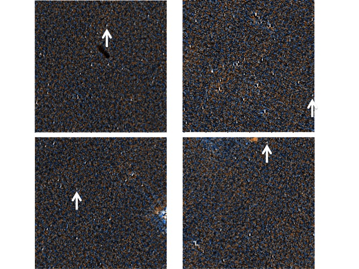
¡En este flipbook, hay “dipolos” en todos lados! ¿Qué significa eso? Si usted ve algo que parece como varios “dipolos” en una imagen, quiere decir que ha habido un problema ligero al direccionar el telescopio. Las estrellas no se movieron; el telescopio sí. Me temo que esos son sólo artefactos. Todos los artefactos estelares tienden a moverse — esté atento a aquellos que se mueven diferente al resto. Dipolos verdaderos (objetos que se mueven lentamente) se ven como dipolos en las cuatro imágenes. Se ven como galletas medialuna, especialmente en la primera y última imagen (excepto que el glaceado blanco puede ser azul o rojo).

¿Es esto un “mover”? Parece un mover pero sólo aparece en dos de las imágenes. Idealmente, un mover real debe aparecer en todas las imágenes. Si un objeto sólo aparece en tres, puede ser un problema con ruido aleatorio, por lo tanto, asuma que es un verdadero mover (y deje que el equipo de científicos decida). Si sólo aparece en dos imágenes, es más probable que sea un artefacto fantasma, no un mover.

¿Qué hago si creo que he descubierto algo? Primero, asegúrese de marcarlo en cada imagen con la herramienta de marcado. Luego, haga un comentario en la página TALK usando el hashtag #mover o #dipole con una descripción sobre dónde ubicar el objeto. Esto le informa a otras personas donde buscarlo dentro de la imagen (ej. “#dipole en rosa claro, esquina superior derecha, R.A. 210.98, dec -22.53”). Luego, revise si se ha publicado previamente en la literatura astronómica usando las herramientas descritas abajo. Si usted encuentra un mover o dipole que no está listado en SIMBAD, ¡por favor llene este formulario! Si no llena el formulario, encontraremos su descubrimiento de todas maneras por las marcas hechas con la herramienta de marcado, pero nos tomará más tiempo ubicarlo e investigarlo.

¡Hice 100 clasificaciones! ¿Por qué no he encontrado nada todavía? ¡Gracias por hacer todas esas clasificaciones! En promedio, debería tomar 60 clasificaciones hasta identificar un objeto con movimiento propio alto conocido. Por supuesto, esos son los objetos que ya conocemos, descubrir algo nuevo tomará dedicación de verdad. Si usted ha hecho 100 clasificaciones y no ha encontrado ningún dipolo o mover, puede ser que esté yendo muy rápido. Tómese su tiempo, mire fijamente cada uno de los artefactos para ver si se mueve de forma diferente en comparación con los demás y asegúrese que el brillo de su monitor esté al máximo. Puede ayudarle dividir mentalmente las imágenes en cuatro cuadrantes y mirar fijamente a un cuadrante a la vez mientras corre la animación; recuerde que, si no encuentra nada, sus clasificaciones aún son útiles: nos informan sobre qué tan comunes o raras son las enanas marrones y cómo restringir búsquedas futuras para el Planeta 9.

¿Cómo uso SIMBAD? SIMBAD (el Set de Identificaciones, Medidas y Bibliografía para Datos Astronómicos, por sus siglas en inglés) es una base de datos de objetos astronómicos muy útil usada por astrónomos profesionales y una herramienta crucial para nosotros en Backyard Worlds: Planet 9. Este blog post explica en detalle cómo usarla para revisar si algún objeto que usted ha encontrado ha sido reportado previamente o si es un descubrimiento nuevo. Aquí le ofrecemos una explicación abreviada.

Una vez que haya usado los números en los lados de la imagen para estimar el R.A. y dec de su objeto favorito, puede consultar SIMBAD en esa ubicación para ver si resulta en objetos astronómicos conocidos. Por ejemplo, digamos que usted vio un objeto interesante en R.A. 277.68 grados y dec 27.545 grados. Vaya a SIMBAD’s coordinate query page, escriba “277.68 27.545” y presione Enter. Note que estas coordenadas son ecuatoriales (FK4 o ICRS) no galácticas ni eclípticas. Le recomendamos fijar el radio de búsqueda en SIMBAD (o VizieR) a 1 minuto de arco. Además, si usted presiona la tecla “i” en un círculo en el título de una página TALK, verá un link hacia SIMBAD que hará una búsqueda de objetos astronómicos en toda la imagen (la búsqueda se da en un radio de 498 segundos de arco a partir del centro del sub-azulejo que está mirando).

Si SIMBAD sólo encuentra una fuente de luz en la imagen que usted está mirando, lo llevará directamente a la página de información sobre dicha fuente. De lo contrario, SIMBAD le mostrará una lista de objetos astronómicos ordenados por su distancia al centro de la sub-azulejo. ¡Haga click en los links para aprender más sobre los objetos que encuentra SIMBAD!

SIMBAD utiliza una larga lista de abreviaturas en sus tablas. Por ejemplo, PM* = estrella de alto movimiento propio, BD* = enana marrón, BD? = candidato de enana marrón, WD* = enana blanca. Puede aprender más sobre SIMBAD en esta guía del usuario.

Una de las características más útiles de SIMBAD es que cada objeto en el catálogo tiene una lista de artículos científicos que mencionan dicho objeto. Si baja a 3/4 de la página, encontrará las “References”. Puede hacer click en “sort references” para ver los títulos de artículos científicos que hayan mencionado o discutido su objeto favorito, si es que hay alguno. Asegúrese de navegar a través de éstos; su objeto favorito puede que sea el foco de un tremendo debate internacional o que haya jugado un rol como calibrador o referencia astrométrica.

¿Cómo uso el Finder Chart? Una tercera revisión que podría hacer sería revisar el NASA IRSA Finder Chart para un campo. Usted encontrará un link en la Finder Chart que mostrará más imágenes de las que mostramos en la herramienta de parpadeo. A diferencia de las imágenes en nuestra página web, las imágenes en el Finder Chart no han sido procesadas para resaltar fuentes de luz que evolucionan con el tiempo. Por esto, usted puede encontrar que un campo que pensó que estaba casi vacío en realidad está bastante lleno.

Finder Chart le mostrará imágenes en varias bandas diferentes: óptica, infrarroja e infrarroja media. Cada una ha sido tomada en un momento diferente. Si su objeto favorito es extremadamente frío (como una enana Y o un planeta), puede ser que no lo vea en ninguna otra imagen aparte de las de WISE. Si el objeto es caliente (como una estrella), puede ser que lo vea en varias décadas, desde imágenes ópticas a infrarrojo medio. Cuando abre Finder Chart, verifique que está viendo el mismo campo que está examinando en nuestra página web fijándose que las mismas estrellas estén en el mismo lugar. Luego, cuidadosamente vea si puede identificar al objeto en otros catálogos (DSS, SDSS, 2MASS, WISE). Haga una anotación en TALK acerca de los catálogos en los que puede ver el objeto. Además, si su objeto es un mover, y si lo puede ver en imágenes de varios catálogos (como 2MASS y WISE), fíjese si puede ver al objeto moverse de una imagen de un catálogo a la siguiente. Luego de este paso, haga una anotación de las fechas de cada imagen y cuantos píxeles (o mejor aún, segundos de arco) se ha movido. La distancia que se ha movido, dividida por la diferencia en tiempo (en segundos de arco por año) nos dice la velocidad tangencial del objeto, un número crucial.

¿Qué son los azulejos y sub-azulejos? El catálogo unWISE divide el cielo en 18,240 “azulejos”. Nosotros hemos dividido cada uno de ellos en 64 “sub-azulejos”, que se convirtieron en las imágenes que usted ve aquí. Sí, son muchos sub-azulejos. El número de sub-azulejo es el número “ID” que aparece cuando le hace click a la “i” en un círculo bajo cada imagen.

¿Cómo uso VizieR? Si usted no puede encontrar lo que busca en SIMBAD, puede usar VizieR para consultar una lista más larga de catálogos astronómicos — ¡casi todos los catálogos que se han publicado! Puede encontrar una introducción a VizieR mucho más detallada en este blog post, aquí le presentamos unas recomendaciones básicas.

Primero, escriba el R.A. y dec de su objeto favorito donde dice “Search by Position” (búsqueda por posición), seleccione una “Target dimension” (“dimensión de objetivo”) de 1 minuto de arco y haga click donde dice “Go”. Alternativamente, cuando haga click en la “i” en un círculo del título de una página TALK, usted encontrará un link a una búsqueda de VizieR de un radio de 498 segundos de arco desde el centro de la imagen.

A diferencia de SIMBAD, VizieR le devuelve MUCHÍSIMAS listas de fuentes, una por cada uno de los catálogos que busca. Cada lista se organiza en orden de distancia de las coordenadas que usted ingresó (ya sean las coordenadas que estimó o el centro del sub-azulejo). Cada catálogo que busca tiene un propósito y condiciones especiales, así que usted deberá leer un poco para utilizar esta poderosa herramienta al máximo. Pruebe en combinar los resultados de una búsqueda para referencias a “proper motion” (movimiento propio), ya que es muy posible que haya identificado una fuente de luz que se ha movido (mover). Ej. Usted puede buscar las letras “pm” en la página web y restringir la búsqueda a objetos con movimiento propio mayor que 100 mas/yr, frecuentemente verá “pmRA” para movimiento propio en ascensión recta y “pmDE” para movimiento propio en declinación. Si encuentra algo que no está en VizieR, por favor anótelo en TALK con el hashtag #notinvizier.

Nota: si usted encuentra su objeto en VizieR pero no en SIMBAD, por favor envíelo al formulario Think You’ve Got One.

Nota: no confíe en los movimientos propios listados en el catálogo AllWISE en VizieR. Son sistemáticamente muy altos. Estamos buscando una razón para ello.

¿Por qué algunas imágenes en este flipbook son negras o parcialmente negras? Hubieron algunos problemas en la misión WISE que imposibilitaron la toma de datos temporalmente y el resultado fue pedazos de cielo donde no hay datos durante algunas épocas, por ejemplo, durante Abril 3, 2004 y Abril 9, 2004, la computadora de la astronave dejó de funcionar correctamente, y la misión tuvo que ponerse en “modo seguro” mientras el comando en Tierra la reiniciaba.

¿Cuáles objetos con movimiento propio se han descubierto previamente? Esta hoja de cálculo lista 3036 objetos conocidos con movimiento propio mayor a 600 milésimas de segundo de arco. Probablemente se encuentre con algunos de estos objetos mientras busca nuevos. Sin embargo, esta lista no cubre todos los posibles dipolos o movers conocidos; usted será capaz de ver dipolos con movimiento propio menor a 200 milésimas de segundos de arco por año, en todo caso, asegúrese de revisar SIMBAD directamente si cree que ha descubierto algo nuevo antes de reportarlo usando el formulario.

¿Qué es esa raya gigante dibujada a lo largo de la imagen? Probablemente es una espiga de difracción asociada con la imagen de una estrella brillante, justo fuera del borde del sub-azulejo al que está mirando. Las espigas de difracción son causadas por luz que se difracta de la estructura de soporte del espejo secundario del telescopio. Las espigas de difracción son la razón por la cual la gente dibuja estrellas con puntas saliendo de ellas. En realidad, las estrellas son más o menos redondas; las puntas o espigas son creadas por telescopios y a veces por nuestros ojos.

¿Qué tan grandes son las imágenes que estoy mirando? Cada imagen tiene 256×256 píxeles y cada píxel mide 2.75 segundos de arco de largo, entonces, las imágenes tienen 704×704 segundos de arco, que equivalen a 11.73×11.73 minutos de arco o 0.195×0.195 grados.

¿Qué hago si veo un mover que se sale del borde de la imagen? Primero, lea el blog post sobre movers rápidos. Luego, si usted decide que este objeto todavía es interesante (ej. Si no es un rayo cósmico u otro tipo de ruido), hay unas cuantas cosas que puede hacer. Primero, márquelo en TALK con los hashtags #mover y #outofframe para que otros puedan hacerle seguimiento, luego, si hace click en el ícono de información en el título de una página de TALK (el i en un círculo en la parte inferior derecha del flipbook), verá “id numbers of nearest subtiles”. Esos números le permitirán buscar los sub-azulejos adyacentes que gustaría revisar.

Para buscarlos, hay dos archivos grandes que va a necesitar. Vaya a https://github.com/marckuchner/byp9 y descargue byp9.subjectnumbers0-583679.csv y byp9.subjectnumbers583680-1167359.csv. La primera columna de cada archivo tiene una lista de los números de sub-azulejos, esos son los números de “Subject ID” de la metadata. La segunda columna tiene una lista de los números de “subject”, esos son números de subject de las páginas web de TALK. Tuvimos que dividir esta tabla de búsqueda en dos archivos, uno para sub-azulejos de números 0-583679, y la otra para números de sub-azulejos 583680-1167359, de otra forma los archivos serían demasiado grandes para descargar. Usted puede buscar cada uno de estos 10 “id numbers of nearest subtiles” en el archivo .csv correspondiente y éste le dirá el número de subject de las páginas web TALK. Coloque uno de estos números al final de la URL de TALK para ir a la página TALK de ser flipbook y así buscar su mover. ¡Disculpe que esto es tan complicado! Estamos tratando de simplificar este proceso.

¿Por qué el R.A y dec de esta imagen están fallados? Los datos de unWISe se guardan usando una proyección gnomónica, que funciona muy bien a través de la mayoría del cielo. Cerca de los polos celestes sur y norte, ¡líneas de R.A. y dec constante ya no corresponden a las líneas rectas de nuestras imágenes! Entonces, a pesar de que las etiquetas de los ejes son técnicamente correctas cerca a los polos, ya no son tan útiles; esto sólo es un problema dentro de un radio de 1 grado alrededor del polo (i.e. para menos de 0.2% de las imágenes). Si usted es suficientemente suertudo para encontrar un objeto interesante en una de estas regiones cerca a un polo, deberá utilizar el Finder Chart para estimar precisamente el R.A. y dec del objeto. Haga click en la i dentro del círculo en una página talk y haga click en el link a la Finder Chart. Luego, mueva el cursor sobre la ubicación correspondiente a su objeto. Las coordenadas aparecerán en la parte superior de su pantalla de Finder Chart. Probablemente encuentre útil hacer click en el botón que dice “Lock By Click” de tal forma que al hacer click en el objeto de una imagen, las coordenadas de ese objeto se muestran incluso cuando usted continúe moviendo el cursor.

¿Cuántos flipbooks hay para clasificar? Tenemos más de un millón de subjects (objetos no clasificados) para clasificar, la mayoría de estos no están online todavía, así que no confíe en el número de “completeness” en la página de destino; ese número solo se refiere al lote de subjects que ya está en línea.

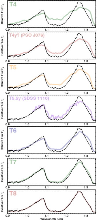
¿Cuándo empezaremos a escuchar resultados sobre el proyecto? Después de hacerle click a un dipolo o mover, o mencionarlo en TALK o enviarlo a través del formulario “Think You’ve Got One”, el siguiente paso para nosotros es investigar ese objeto y averiguar lo que ya se sabe de él. Luego tenemos que aplicar a tiempo de telescopio para hacerle seguimiento a los objetos más interesantes para tomarles un espectro. Los espectros de luz nos ayuda a averiguar sus tipos espectrales y sus temperaturas, e identificar si lo que estamos viendo es realmente una enana marrón o un planeta. Todo ese proceso generalmente toma meses. Para tener las últimas actualizaciones, ¡síganos en Facebook o en Twitter @backyardworlds!

Preguntas Generales de Astronomía

¿Cuál se supone que es la apariencia de Planet 9? La Field Guide contiene simulaciones de cómo se podría ver Planet 9, y aquí hay un blog post crucial con detalles sobre los patrones característicos del planeta que siguen un movimiento JUMP JUMPBACK, y JUMP hop JUMP hop. Su color depende de cuánto metano contiene su atmósfera. De acuerdo a los modelos de Fortney et al. 2016, Isi el planeta tiene una composición similar a la del Sol, con gas metano en su atmósfera, será más brillante en la banda WISE 2, así que se verá rojo en los flipbooks. Si el metano se ha congelado en su atmósfera, que parece probable, el planeta se verá más brillante en la banda WISE 1 y se verá azul en los flipbooks. También es posible que el planeta sea muy pequeño y oscuro como para verse en nuestros datos. En todo caso, debería ser un mover y debería moverse rápido, probablemente la mitad o todo el camino a través del flipbook, mientras usted observa. Note que su movimiento de saltos en el flipbook será más o menos horizontal.

¿Qué son variables Mira? Muchos de los objetos más brillantes que verá en Backyard Worlds: Planet 9 son gigantes rojas, que a veces pulsan. Para hacer las imágenes que usted ve en esta website, restamos una época de la otra, lo que causa que las estrellas variables destaquen. Si usted ve un artefacto estallar enorme como el presentado arriba, es probable que sea una gigante roja pulsante. Las variables Mira son un tipo de gigante roja pulsante. Estas estrellas gigantes y frías se convierten cien veces más brillantes y luego débiles otra vez durante un período de un año aproximadamente.

¿Cómo se ven las enanas marrones? Se conoce que las enanas marrones son más brillantes en las bandas WISE 2 (4.6 micrones) que en la banda WISE 1. Entonces se ven rojas o blancas en nuestra escala de color. Pueden ser movers o dipolos.

¿Quién más está buscando al Planet 9? Varios otros grupos están buscando a Planet 9. La Dark Energy Survey utiliza un telescopio en el Observatorio Interamericano del Cerro Tololo. La survey Pan-STARRS utiliza un telescopio dedicado en Mt. Haleakala en Hawaii. El telescopio Subaru en Hawaii también está haciendo una búsqueda más profunda pero altamente colimada. La survey SkyMapper utiliza un telescopio en el Observatorio de Siding Spring en Australia; esta survey es la base para otro proyecto de Zooniverse llamado simplemente “Planet 9”.

Todas estas otras surveys están buscando en longitudes de onda ópticas utilizando telescopios basados en Tierra, mientras que nosotros en Backyard Worlds: Planet 9 estamos buscando en longitudes de onda infrarrojas utilizando un telescopio en el espacio. Esto nos permite buscar en todo el cielo, en vez de estar limitados a un pedazo de cielo. Nadie sabe todavía si Planet 9 será más brillante en las ondas infrarrojas en las que estamos trabajando o en ondas ópticas donde trabajan las otras surveys, entonces tiene sentido buscar en ambas partes del espectro. Lea el blog post de Aaron Meisner para aprender más.

¿Podrían haber planetas más allá del Planet 9? Es posible que hayan más planetas aún no descubiertos en órbita alrededor del Sol, además de Planet 9. Volk and Molhotra (2017) sugirieron recientemente que un décimo planeta podría ser responsable por causar una deformación del plano del cinturón de Kuiper. Este pequeño planeta probablemente sea muy débil para detectarlo aquí en Backyard Worlds: Planet 9. Del mismo modo, otros planetas podrían estar al acecho más allá de las presuntas órbitas del noveno o décimo planeta. Sin embargo, no hay evidencia en particular que favorezca a un onceavo planeta, como sí la hay para un noveno planeta.

¿Por qué nos importan las enanas marrones? Las enanas marrones son el vínculo entre la formación de estrellas y la de planetas. Tienen características físicas comunes entre estrellas y planetas. Contando el número de objetos que hay y determinando sus masas, podemos aprender sobre cómo se forman los planetas, estrellas y galaxias. Las enanas marrones frías son particularmente útiles porque las usamos como análogos a exoplanetas. Son del mismo tamaño que Júpiter y a veces la misma temperatura que Júpiter o incluso, la Tierra, pero son mucho más fáciles de estudiar que los exoplanetas porque éstas no orbitan estrellas brillantes que las opacarían con su brillo. Como consecuencia, podemos obtener información muy detallada sobre sus atmósferas, lo cual nos informa acerca de su composición, rotación, nubes, tormentas e incluso propiedades magnéticas. Algunas enanas marrones incluso tienen planetas que las orbitan. Trabajando con usted en este proyecto de ciencia ciudadana, esperamos descubrir enanas marrones exóticas con características de nubes que nos ayuden a entender la diversidad de atmósferas encontradas en exoplanetas. Para aprender más, lea el blog post de Jackie Faherty.

¿Cuántas enanas marrones esperamos encontrar? Tenemos una idea razonable sobre cuántas estrellas y enanas marrones hay cerca al Sol con tipos espectrales L2 y más tempranos (más calientes), pero la mayoría de éstas probablemente ya se han encontrado. Los tipos tardíos (más fríos) se mantienen misteriosos. ¡Uno de nuestros goles principales en Backyard Worlds: Planet 9 es resolver esta pregunta sobre qué tan comunes son las enanas marrones más frías!

En 2012, Kirkpatrick et al. estimó que hay 5 enanas marrones con tipos T6-T8.5 y por lo menos 6 de tipos T9 y más tardíos (más frío) a menos de una distancia de 7 parsecs a partir del Sol. Luego Luhman (2014) descubrió un nuevo objeto llamado WISE J085510.83-071442.5 que rompió el récord de la enana marrón más fría, y eso forzó a la gente a rehacer sus estimaciones. Desde ese entonces, Zapatero Osorio et al. 2016 estima que debe haber entre 15 y 60 enanas marrones de tipo Y2 dentro del volumen de 7 parsecs alrededor del Sol. Mientras tanto, Yates et al. 2016 predijo que dentro de 10 parsecs alrededor del Sol, hay 3 enanas tipo Y con tipos entre Y0 e Y0.5, y solo uno con un tipo más tardío (más frío, como Y1 o Y2). Cómo puede ver, el amplio rango de estimaciones surge porque se hacen extrapolaciones de una lista conteniendo solamente unos cuantos objetos.

¿Cuántas enanas marrones se conocen hoy en día? Miles. dwarfarchives.org actualmente enumera 1281 enanas marrones de tipo L y T (hasta 2012). Sin embargo, sólo 24 enanas marrones son de tipo Y (a temperatura ambiente) y sólo 3 se encuentran a 10 años luz o menos del Sol. Esperamos encontrar más de estos objetos raros y cercanos.

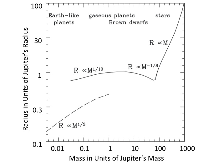
¿Qué son enanas de tipos M, L, T e Y? Al igual que las estrellas, las enanas marrones se clasifican por las líneas de absorción en sus espectros, que son indicadores de su temperatura superficial. Las enanas M tienen una temperatura de 3500-2100 K, las enanas L de 2100-1300 K, las T de 1300-600K y se cree que las enanas Y son más frías que 600K. Como casi todas las enanas marrones tienen el mismo tamaño físico, a menor temperatura, menor brillo emite el objeto. Los “tipos” de enanas marrones son una continuación de la secuencia de tipos estelares; la lista completa es O, B, A, F, G, K, M, L, T, Y. Cada tipo tiene subtipos, indicados por números, que describen variaciones más sutiles en temperatura, por ejemplo, una enana T6 es más fría que una enana T3. Tanto las estrellas como enanas marrones pueden ser enanas M; las enanas marrones no son generalmente más calientes que una M6. Acá hay una reseña científica de Adam Burgasser con más información.

¿Cuál es la enana marrón más cercana? Un par de enanas marrones llamadas Luhman 16 o WISE J1049-5319, que se ubica a 6.52 años luz (1.99 parsecs) del Sol; son las enanas marrones conocidas más cercanas. Probablemente usted descubrirá una que está aún más cerca. Este diagrama (crédito: NASA/Penn State University) muestra las ubicaciones de las enanas marrones y estrellas más cercanas al Sol.

¿Cuál es la estrella más cercana al Sol? Proxima Centauri es la estrella más cercana al Sol. Parece ser el miembro más débil de un sistema de tres estrellas llamado Alpha Centauri, así que también se conoce como Alpha Centauri C. ¿Le parece extraño que la estrella más cercana esté más cerca que la enana marrón más cercana? A nosotros sí…

¿Podemos ver planetas en el Cinturón de Kuiper u otros objetos del Cinturón de Kuiper en estas imágenes? No, son muy débiles en estas longitudes de onda.

¿Qué significa MJD? MJD son las siglas en inglés para Modified Julian Date (Fecha Juliana Modificada), el número de días desde la medianoche del 17 de Noviembre de 1858. Cada imagen astronómica en esta página web tiene una estampilla de tiempo con una Fecha Juliana Modificada indicando cuándo se tomó.

WiseView

This week, I’m excited to present this guest post from two of our users, Dan Caselden and Paul Westin. They wrote their own tool for viewing the WISE data, called “WiseView”. It provides some useful options you won’t find at the backyardworlds.org site. Enjoy!

Marc Kuchner

As you may know, the images at ByW: P9 all ultimately come from a database called unWISE, which is a project that reprocesses WISE single exposures to generate coadded images with improved clarity. Since we citizen scientists with ByW: P9 are always eager to know more about our subjects, we found ourselves often visiting the unWISE site to obtain different views of our favorite patches of sky.

However, we felt that unWISE’s packaging could stand to be a little more user friendly. So, after a while, we decided to add a friendly wrapper, to make this data easier to examine, and share it with you. We’re a far cry from User Interface/User Experience professionals, but, hey, it’s a start!

Our tool, wiseview (http://byw.tools/wiseview), displays two sets of cutouts (i.e., portions of larger images of the sky). At the top, wiseview flashes coadded imagery from the WISE satellite. These cutouts come from unWISE. unWISE currently contains coadded images for three data sets: AllWISE, NeoWISE-R1, and NeoWISE-R2. unWISE coadds are full-depth. That is, unWISE NEO1 also incorporates the single exposures used by unWISE AllWISE, and unWISE NEO2 also incorporates the single exposures used by unWISE NEO1 and unWISE AllWISE. Consequently, particularly high proper motion options will appear to stretch, or even fade in one position and appear in another.

Since ByW: P9 participants are on the hunt for things that move in WISE data, unWISE images are a natural resource for further investigation. After identifying coordinates of a pattern possibly indicative of proper motion, participants can zoom in with wiseview to see a closer representation of the underlying data from the flipbooks. The “field of view” parameter selects what size cutouts to display, in arcseconds, and the zoom slider blows up the unWISE cutouts. WISE W1 and W2 bands can be isolated with the WISE band field (W1 for W1, W2 for W2, and W1+W2 for both), and the “Speed” slider changes how quickly the cutouts flash.

The second cutout is a composite image from PanSTARRS-1, created in the same way as the default PanSTARRS-1 cutouts: band y colors red, band i colors green, and band g colors blue. PanSTARRS-1 cutouts are great for comparison versus unWISE because many unwanted sources and some of the brighter and/or earlier brown dwarfs show distinguishably.

unWISE Post-Processing

unWISE cutouts are normalized with astropy.visualization.AsinhStretch, and mapped to a colormap with matplotlib. The following images show AsinhStretch applied to a greyscale gradient with differing values of ‘a’. The ‘Linear’ parameter in wiseview is directly passed through to this parameter in AsinhStretch. ‘Linear=1.0’ applies a purely linear normalization to the image, which has no effect.

Images3-5

Lower values highlight lower intensity pixels, which is useful for observing faint sources, or those obscured by other, brighter, sources. For example, The images below show Ross 458C with varying values of ‘Linear’.

Images6-8

However, purely AsinhStretch normalization can make modest proper motions difficult to discern. Observationally, the normalization appears to lose dynamic range at the edges of sources, which is where the eye seems to most perceive motion in these images.

The three modes, ‘fixed’, ‘percent’, and ‘adapt’, attempt to compensate for this by capping intensity ranges before AsinhStretch normalization. ‘fixed’ caps the maximum intensity to an absolute number supplied by the slider ‘Trim Bright’. ‘percent’ caps the maximum intensity to a percentile within the image, again using the slider ‘Trim Bright’. ‘adapt’ is very much a work in progress that (poorly!) attempts to find a good intensity range automatically.

Why wiseview?

We wrote wiseview to improve our accuracy (and sate our curiosity!) when classifying candidates in the ByW: P9 flipbooks. With wiseview, curious participants can investigate their subjects to show whether their candidates demonstrate proper motion. For particularly challenging candidates that are not easily distinguishable in other available imagery like 2MASS, comparing unWISE coadds can be our only option to demonstrate proper motion.

Although we originally wrote wiseview for use with ByW: P9, its applications are more general; anyone searching near-infrared for objects in the solar neighborhood may find it helpful. In fact, multiple ByW: P9 participants discovered candidates in side projects using wiseview.

By the way, if you’re interested in unWISE, another great resource is legacysurvey.org’s Sky Viewer. For getting a quick big picture of what’s going on in a portion of the sky and disambiguating sources, their tool is invaluable. It also provides other image sets and catalog overlays, like DECaLS and SDSS, if your coordinates are lucky enough to fall within those surveys. Very nice!

Thank you!

We are Dan Caselden and Paul Westin, two computer security researchers from California with absolutely zero background in Astronomy. Thanks for reading!

First Observing Proposal of the Season

Fall is just around the corner here in the northern hemisphere, so it’s the time of year when we write observing proposals! And last week, we submitted the first Backyard Worlds: Planet 9 proposal of the season–to follow up some of our brown dwarf candidates using the Astrophysical Research Consortium (ARC) 3.5 meter telescope at Apache Point Observatory. We asked for half a night of time on Near-Infrared Camera & Fabry-Perot Spectrometer (NIC-FPS), to perform J band photometry of 10 objects. Photometry means you take a picture of the object and sometimes a picture of a reference star, and you use the image to figure out how bright your object is. J band corresponds to a wavelength of light of about 1.25 microns, about the size of a virus or a particle of soot.

Image result for apache point observatory arc 3.5 — ARC 3.5 meter telescope at Apache Point Observatory, New Mexico.

Here’s why we we need these brightness measurements (the photometry). While many of our brown dwarfs have infrared photometry from surveys like 2MASS and Pan-STARRS, the reddest, coldest, and probably the most interesting objects are too faint for these surveys! 2MASS went as faint as about 16th magnitude in J band. Pan-STARRS data goes down to about 21st magnitude in y band (a wavelength of around 1.02 microns). But ultracool brown dwarfs are faint, faint, faint. So we need to make our own measurements.

Once we have the new photometry, we will be able to do two new things. First, we will be able to get much better estimates of the spectral types of these objects. As you may recall, the spectral type of the coldest brown dwarfs is Y. Only 25 Y dwarfs are presently known. T dwarfs are the next coldest, but hundreds of T dwarfs are have already been discovered, so Y dwarfs are much more exciting. So far, all we know about the targets we have in mind is that they have WISE colors that are similar to those of Y dwarfs (i.e. brighter in W2 than W1 by at least 2.5 magnitudes). But they might still turn out to be late T dwarfs. The near infrared photometry will help make that distinction.

Second, we will be able to apply for time on still larger telescopes to get their near-infrared spectra. The photometry will tell us what instrument we will need, and how long we need to keep the shutter open while were are collecting the spectra. These spectra will tell us for sure what the spectral type is (Y or T?), and maybe even lead to a big discovery.

Here’s a link to the full proposal, if you are curious: APO_BWs The final target list is not set yet, but the 10 targets that meet our cutoff of W1-W2 > 2.5 were found by Guillaume Colin, Sam Goodman and Dan Caselden. Nice work, guys!

I’m sure we’ll be writing several more telescope proposals over the next month—stay tuned!

Marc

A Guide to Classifying on Backyard Worlds: Planet 9 from the Point of View of a Citizen Scientist

Enjoy this guest post by one of our moderators, Michaela Allen, featuring a video by Guillaume Colin!

Hello newcomers to Backyard Worlds: Planet 9! Or maybe you are a returning citizen scientist to this project… whatever the case, welcome! My goal for this post is to give you a basic beginner’s guide to classifying objects on BW (Backyard Worlds: Planet 9). I am in NO way an expert, but I’d like to share what I have learned so far so that maybe you can learn something too!

A little about me first… My name is Michaela Allen, (@mallen33 on Zooniverse) and I am a current college undergrad student studying physics and astronomy. I’ve been helping classify objects on BW since the project launched, and I’ve learned so much since then! Going into this project I had no idea what it entailed—I was just excited at the prospect of potentially finding something that hadn’t been discovered before!

The first thing I want to share with everyone is a YouTube video made by fellow citizen scientist Guillaume Colin (@karmeliet on Zooniverse) all about his method of analyzing flipbooks on BW. This is a great video where he talks about the basics of BW, SIMBAD, and IRSA. He also goes through the steps of filling out the Think-You’ve-Got-One Form, which can be tricky to find all of the information needed for the form. Seriously, go check it out, and thanks to Guillaume for making this video!

Now, for the rest of this post, we going to look at some of my favorite subjects on BW. So let’s get started!

When you first go on BW, you get to go through a tutorial that shows you all kinds of examples of dipoles, movers, artifacts, etc. You also have a handy field guide on the right of the screen that shows examples of these as well. The tutorial and the field guide are great references to go back and look at– do not forget to use them! I still reference back to them all the time. While those are great examples to get started with, classifying your first subject can still be kind of overwhelming! I’d like to give y’all a few more examples of types of objects and subjects you may encounter while classifying.

In terms of fast movers, I haven’t come across any (yet!). The example in the field guide of Y Dwarf WISE 0855-0714 is what I still go off of. And remember, a true fast mover will appear in all four frames of a subject.

This subject contains a type of artifact called a ghost—it only appears in two frames. These ghosts are not movers and do not need to be submitted to the Think-You’ve-Got-One form.

Other mover “imposters” to look out for is extra noise surrounding the area of declination of the South Atlantic Anomaly. This is in the -25 degrees region of declination, give or take a few arcminutes. This anomaly, which Marc talks more about in his Fast Movers post, tends to cause more noise in the subjects—and the noise can often look a lot like fast movers. For example, take a look at this subject.

There are a few orange dots visible throughout the frames that do look deceivingly like fast movers, but they are just noise. The area of declination and the often sporadic movement of these dots give away that these are not movers.

In terms of dipoles or slow movers, I have seen many! Some are definitely easier to spot than others. A dipole is an object that is moving but in a different way to all of the other objects in the subject. This subject is one of the first subjects I classified on BW, and it has a dipole! See if you can find it.

There it is at RA 151.99, dec 25.51 . I think this one is a great example of a lot of the dipoles I have seen. It isn’t super bright, but it’s not too faint either. It immediately stuck out to me, so I commented on the TALK page and asked for other opinions– don’t forget to comment on the talk pages too! If you’re ever unsure about anything, TALK about it (pun intended)! Sure enough, some people commented back, and I had found my first dipole!

Now, they aren’t all as easy to spot as this one. Faint dipoles take a little more effort. And remember, the fainter a dipole, the better of a chance it has of not being discovered! See if you can find the faint dipole in this subject.

This one is at RA 161.21, dec 13.79— to the right of that artifact. In terms of bigger and brighter dipoles, most of them I have seen have been in SIMBAD and are high proper motion stars. But just because it is bigger and brighter doesn’t mean it is going to be in SIMBAD! Always check to make sure!

Now sometimes you may find multiple objects of interest in a subject, which is great! You have to be careful of misalignment errors sometimes, though. These errors, caused by slight movements of the telescope, make the subjects seem like there are multiple dipoles. We talked about this subject, mentioned by another citizen scientist, @Chrismkemp, in one of the BW hangouts. She had seen seven or eight dipoles in this one subject and was wondering if that was even possible. I’ve come across subjects like these a few times, and they can be pretty tricky to classify. Do you see how the “dipoles” seem to kind of elongate? Marc calls them petals. Unfortunately, they can’t actually be classified as dipoles. If you ever have a subject that seems as if it has multiple dipoles, look for this “petal effect”. There was one real dipole in this subject, though. See if you can spot it!

That real dipole is at RA 349.77 dec -53.63 . This object one doesn’t seem to grow petals like all of the other imposter “dipoles” do in this subject.

The last thing I have to share with y’all is bad frames in some of the subjects. These can range anywhere from stripes across the frame, completely black frames, to half of the frame being cut off like in frame 3 of this subject. While these frames may sometimes look interesting, they do not need to be reported. If you ever come across them, you can always add the #badimage hashtag on the talk page.

Well, I hope that my limited experience has helped some of y’all on classifying objects at Backyard Worlds: Planet 9. Thanks to Marc for letting me share with everyone here! I’ve loved getting to participate in this project, and I’m excited to continue working on it!

See you on TALK, and happy hunting!

-Michaela Allen

Our First Paper: the Discovery of Brown Dwarf WISEA 1101+5400

Our first paper was published in the Astrophysical Journal Letters, Volume 841, Number 2 on May 24. Hooray!! (It may be easier to read here.)

The paper announces the discovery of our first brown dwarf, shows a spectrum we took of the brown dwarf, and describes the Backyard Worlds: Planet 9 project. There’s a press release from the American Museum of Natural History, a nice NPR story about it featuring Rosa Castro, and several other news stories.

Of course, this paper is already out-of-date. In the time it took to write the paper, you’ve discovered at least twelve more good brown dwarf candidates. And we used those discoveries to make an even better estimate of the sensitivity of our search than the one that appears in the paper. But let’s talk more about the paper and our first discovery, a source called WISEA 1101+5400 which we now know is a real brown dwarf, spectral type T5.5. Here is WISEA 1101+5400’s flipbook.

You may recall that shortly after launch, we were all excited about a faint dipole/mover, which Bob Fletcher had flagged on talk and Tamara Stajic reported on the Think-You’ve-Got-One form. That’s WISEA 1101+5400. A few weeks later, science team member Jackie Faherty nabbed a spectrum of it using NASA’s Infrared Telescope Facility. Here’s a nice plot of the spectrum, created by science team member Joe Filippazzo comparing the our object’s spectrum (black) to the spectrum of another T5.5 brown dwarf (red). It’s a great match! The extra wiggles in our spectrum are simply noise.

Figure3.cropped

The quality of the match demonstrates that WISEA 1101+5400 is indeed a brown dwarf, and tells us that its temperature is in the range 900-1500 Kelvin (1200 – 2200 degrees Fahrenheit). We can tell the temperature range by looking at what molecules show up in the spectrum. The spectrum shows features associated with water, methane, iron hydride, potassium, and molecular hydrogen, labelled above. If the brown dwarf were hotter or cooler, the relative sizes of the dips in the spectrum from each molecule would be different.

Knowing the brown dwarf’s spectral type also teaches us roughly how bright it is, intrinsically. And since we know that the brightness of an astronomical object falls off as the inverse distance to it, squared, we can compare our images of WISEA 1101+5400 to those of other brown dwarfs to estimate its distance: roughly 34 parsecs or about 111 light years. For comparison, the closest known brown dwarf is the binary Luhman 16AB at 6.59 light years.

So what does this discovery mean for our understanding of brown dwarfs? Well, there are already a few hundred T dwarfs known–and this new one turns out to be somewhat run-of-the mill. It’s not super cool, and it’s not in a moving group, for example. Its infrared colors are close to the average colors for brown dwarfs with this spectral type. So we haven’t shattered any paradigms or broken any records with this object just yet.

But the discovery is a dramatic proof-of-concept. Just the fact that we found it, only six days after launch, shows that we’re on the right track toward lots more discoveries. Also, Zooniverse founder Chris Lintott tells me that our paper now holds the record for fastest publication from a Zooniverse project. How cool is that?

This is a moment to celebrate. Congratulations to us!! Let’s make some more discoveries and write some more papers together.

Marc

We’re up to twelve brown dwarf candidates now, plus one real verified brown dwarf!

Hey everyone! It’s proposal season here at NASA. Every spring, NASA offers astronomers opportunities to apply for grant funding to do their research, and we’ve been busy taking advantage of that, writing proposals.

In the meantime, you’ve been hard at work, discovering stuff. We’re up to twelve brown dwarf candidates now plus one real verified brown dwarf. Holy smoke! We can estimate their spectral types based on their relative flux in the WISE 1 and WISE 2 bands (3.5 and 4.6 microns), and it looks like we have 7 new candidate L dwarfs and five new candidate T dwarfs. We’re going to try to get spectra for as many of these as we can.

In the meantime, did I mention we’ve been writing proposals? Well in a proposal, you try to make predictions about what you’re going to be able to learn or discover. You also try to show how your work compares to other work in the field. So we started by taking all thirteen objects and putting them on a plot, showing their proper motions and magnitudes in the WISE 2 (W2) band. Those are the red stars on the plot below, which was made by science team member Jonathan Gagne.

PM_relW2_BYW

Then, as you can see, we plotted lots of other interesting stuff on here. For starters, we did our best to add all the brown dwarfs that were previously known. The little blue dots show every other brown dwarf in this database, which is every brown dwarf we could find in the literature. You can see right away that our discoveries, the red stars, fall towards the bottom of the cloud of blue dots made by the other discoveries. So our discoveries are fainter than average.

Next, we plotted some lines indicating the detection limits of some other recent surveys, by Adam Schneider et al and by Davy Kirkpatrick et al. (That’s Adam Schneider from our science team.) Those are the two biggest brown dwarfs searches made using WISE before we began ours. The survey done by Schneider et al. only detected brown dwarfs that fall above the orange dashed line. The survey done by Kirkpatrick et al only detected brown dwarfs that fall above the black dash-dot line. Those lines slant upward to the right because the WISE images they used were not divided into as fine time slices as ours, so some faster moving objects got blurred out.

Finally, we added some green lines showing what we think are the limits of Backyard Worlds: Planet 9. Now this part is harder since our survey, of course, isn’t complete yet. But we do know more or less what the shapes of the curves should be. We know that they slant up on the left side of the plot because that’s where the motion is too slow and the images of a moving object start self-subtracting. And we know that the objects we have already detected, the red stars, must lie above the lines. So we draw the curves and shift them around till they hug the bottom of the cluster of red stars—and that’s our best guess at our detection limits.

Note that there are two green lines. That’s because WISE spent more time making images at higher latitudes (here the symbol, beta, means latitude), so our survey is a bit more sensitive there. There’s only one brown dwarf candidate that’s up at a high latitude where this effect comes into play, though—it’s the one sitting on the lower green line.

So there we have it: a prediction for the sensitivity of our search. We will spot any brown dwarfs that fall above the green lines (pick the right one based on latitude). And we are the first to make an all-sky survey of the region above the green lines and below the orange and black lines. (A few brown dwarfs are already known in this region, but they came from surveys that only covered relatively small portions of the sky).

Now, remember that this plot uses logarithmic scales! Each of the big ticks on the x axis is a factor of 10. Each magnitude (the y axis) represents a factor of about 2.512. So that space on the plot could contain lots of brown dwarfs and other interesting objects, especially at high proper motions. Good luck!

Marc Kuchner

More Discoveries: New Candidate L Dwarfs!

Good work, everybody! You’ve submitted at least five good newly discovered candidate L dwarfs on the Think-You’ve-Got-One form.

Let’s talk about L dwarfs. The L spectral type contains object with temperatures in the range of about 1400-2200 Kelvin. It was first established in 1999 by Kirkpatrick et al.. They chose the letter “L” because it is next to “M” in the alphabet; M was the coolest spectral type in the literature at the time, and “N” was already taken to describe a class of evolved stars. Amazingly, L dwarfs are about twice as common as main sequence stars. They are just harder to spot because they are so much more faint and red.

The first L dwarf discovered was GD 165B, found by Becklin & Zuckerman in 1988. Curiously, 165B orbits another special kind of astronomical object: a white dwarf. Nowadays, about 1300 L dwarfs are known. So discovering one new one doesn’t usually merit a paper on its own. But when we collect a batch of 50 or so we will definitely want to announce them with a publication, especially if one or more turn out to be in moving groups of young stars. For example, here’s a recent paper by our own Adam Schneider announcing the discovery of 47 new L dwarfs, including seven that are in young moving groups. Membership in a moving group is important because it establishes the objects age.

A good clue that you might have an L dwarf is if it doesn’t appear in the DSS images, only in 2MASS and WISE. That’s because the DSS images were taken in visible wavelengths, and L dwarfs are too cool to shine in visible light, so they only show up in 2MASS and WISE bands, which are infrared. (T and Y dwarfs may not even show up in the 2MASS images). Just remember, the rule of thumb is that if it’s not in SIMBAD, we want to see it on the Think-You-ve-Got-One form. There are still interesting objects to find that are in DSS images.

Here’s one of the ones you found. It’s a great test for the eyes!

Ldwarf.x2.y1

It’s a faint bluish dipole. Can you spot it in this flipbook? If not, scroll down to the answer key at the end of this article.

Here’s another one. Remember, each one of these is a real new discovery–not a recovery of an object that was known before!

Ldwarf.x7.y6

Can you see it there? Here’s a third on to challenge yourself with.

Ldwarf.x4.y1

OK here’s one more for you to test your skill on…

Ldwarf.x6.y4

Ignore that giant blinking blue ghost in the middle! They are tough to spot. If you need help, here are the answers, below. Congratulations to @Andy_Arg, @karmeliet, @graham_d, @stevnbak, and @NibiruX for their exceptional eyesight And keep up the good work, everybody!!

LdwarfFinder

Marc Kuchner